1강: 표현형 기반 임상 데이터 기초 통계 분석

BBP WGS 분석 튜토리얼

학습 목표

표현형 기반 임상 데이터 구조 이해 - 1000 Genomes Project의 샘플/표현형 데이터 구조를 파악
임상 정보 통계 및 연관성 분석 - 인구집단별, 성별 등 임상 변수의 기초 통계 및 연관성 분석
유전변이(VCF)-임상 표현형 통합 분석을 위한 전처리 - VCF 데이터와 임상 데이터를 결합하기 위한 데이터 정제

사용 데이터

데이터 루트: /tier4/DSC/jheepark/bbp-wgs-data/

데이터	경로	설명
샘플 패널 정보	`phenotype/integrated_call_samples_v3.20130502.ALL.panel`	2,504 샘플의 population / super_population / gender
샘플 상세 정보	`phenotype/20130606_sample_info.xlsx`	샘플별 상세 메타데이터 (시퀀싱 플랫폼, 커버리지 등)
Pedigree (가계도)	`phenotype/20130606_g1k.ped`	가족 관계, 성별, 표현형 정보 (PED 형식)
1000 Genomes chr22 VCF	`individual/ALL.chr22.phase3_shapeit2_mvncall_integrated_v5b.20130502.genotypes.vcf.gz`	VCF 샘플 목록 매칭 검증용

산출물 (본 강의에서 생성)

파일	경로	설명
통합 샘플 정보	`phenotype/integrated_sample_info.tsv`	Panel + VCF 샘플 순서 병합 (2–4강에서 재사용)
EAS 서브셋	`phenotype/eas_sample_info.tsv`	동아시아(EAS) 504 샘플
Unrelated 샘플 목록	`phenotype/unrelated_samples.txt`	부모 정보 없는 unrelated 샘플 ID (4강 GWAS용)

사용 도구

Python: pandas, numpy, matplotlib, seaborn, scipy
bcftools (VCF 샘플 목록 확인용)

0. 환경 설정

python

import pandas as pd
import numpy as np
import matplotlib.pyplot as plt
import seaborn as sns
from scipy import stats
from matplotlib import font_manager, rc
import warnings
warnings.filterwarnings('ignore')

# 시각화 설정 (seaborn 스타일을 먼저 설정해야 한글 폰트가 덮어씌워지지 않음)
sns.set_style('whitegrid')
sns.set_palette('Set2')

# 한글 폰트 설정 (seaborn 설정 이후에 적용)
font_path = '/usr/share/fonts/truetype/nanum/NanumGothic.ttf'
font_manager.fontManager.addfont(font_path)
rc('font', family='NanumGothic')
plt.rcParams['axes.unicode_minus'] = False  # 마이너스 기호 깨짐 방지
plt.rcParams['figure.figsize'] = (12, 6)
plt.rcParams['font.size'] = 12

# 데이터 경로 설정
DATA_DIR = '/tier4/DSC/jheepark/bbp-wgs-data'
PHENOTYPE_DIR = f'{DATA_DIR}/phenotype'
INDIVIDUAL_DIR = f'{DATA_DIR}/individual'

print('환경 설정 완료!')

환경 설정 완료!

1. 표현형 기반 임상 데이터 구조 이해

1000 Genomes Project는 전 세계 26개 인구집단에서 2,504명의 개인을 대상으로 whole genome sequencing을 수행한 대규모 유전체 프로젝트입니다.

1.1 샘플 패널 데이터 로드

.panel 파일은 각 샘플의 인구집단(population), 대륙 그룹(super population), 성별(gender) 등 기본 정보를 담고 있습니다.

python

# 샘플 패널 정보 로드
panel = pd.read_csv(
    f'{PHENOTYPE_DIR}/integrated_call_samples_v3.20130502.ALL.panel',
    sep='\t'
)

print(f'전체 샘플 수: {len(panel)}')
print(f'컬럼: {list(panel.columns)}')
print()
panel.head(10)

전체 샘플 수: 2504
컬럼: ['sample', 'pop', 'super_pop', 'gender', 'Unnamed: 4', 'Unnamed: 5']

	sample	pop	super_pop	gender	Unnamed: 4	Unnamed: 5
0	HG00096	GBR	EUR	male	NaN	NaN
1	HG00097	GBR	EUR	female	NaN	NaN
2	HG00099	GBR	EUR	female	NaN	NaN
3	HG00100	GBR	EUR	female	NaN	NaN
4	HG00101	GBR	EUR	male	NaN	NaN
5	HG00102	GBR	EUR	female	NaN	NaN
6	HG00103	GBR	EUR	male	NaN	NaN
7	HG00105	GBR	EUR	male	NaN	NaN
8	HG00106	GBR	EUR	female	NaN	NaN
9	HG00107	GBR	EUR	male	NaN	NaN

python

# 데이터 기본 정보 확인
print('=== 데이터 타입 ====')
print(panel.dtypes)
print()
print('=== 결측치 확인 ====')
print(panel.isnull().sum())
print()
print('=== 기초 통계 ====')
panel.describe(include='all')

=== 데이터 타입 ====
sample         object
pop            object
super_pop      object
gender         object
Unnamed: 4    float64
Unnamed: 5    float64
dtype: object

=== 결측치 확인 ====
sample           0
pop              0
super_pop        0
gender           0
Unnamed: 4    2504
Unnamed: 5    2504
dtype: int64

=== 기초 통계 ====

	sample	pop	super_pop	gender	Unnamed: 4	Unnamed: 5
count	2504	2504	2504	2504	0.0	0.0
unique	2504	26	5	2	NaN	NaN
top	NA21144	GWD	AFR	female	NaN	NaN
freq	1	113	661	1271	NaN	NaN
mean	NaN	NaN	NaN	NaN	NaN	NaN
std	NaN	NaN	NaN	NaN	NaN	NaN
min	NaN	NaN	NaN	NaN	NaN	NaN
25%	NaN	NaN	NaN	NaN	NaN	NaN
50%	NaN	NaN	NaN	NaN	NaN	NaN
75%	NaN	NaN	NaN	NaN	NaN	NaN
max	NaN	NaN	NaN	NaN	NaN	NaN

1.2 Super Population (대륙 그룹) 이해

1000 Genomes Project는 5개의 대륙 그룹(Super Population)으로 분류됩니다:

AFR: African (아프리카)
AMR: Ad Mixed American (아메리카 혼혈)
EAS: East Asian (동아시아)
EUR: European (유럽)
SAS: South Asian (남아시아)

python

# Super Population별 샘플 수
superpop_counts = panel['super_pop'].value_counts()
print('=== Super Population별 샘플 수 ===')
print(superpop_counts)
print()

# Population별 샘플 수
pop_counts = panel['pop'].value_counts()
print('=== Population별 샘플 수 ===')
print(pop_counts)

=== Super Population별 샘플 수 ===
super_pop
AFR    661
EAS    504
EUR    503
SAS    489
AMR    347
Name: count, dtype: int64

=== Population별 샘플 수 ===
pop
GWD    113
YRI    108
IBS    107
TSI    107
CHS    105
PUR    104
JPT    104
CHB    103
GIH    103
ITU    102
STU    102
ESN     99
CEU     99
LWK     99
FIN     99
KHV     99
PJL     96
ACB     96
CLM     94
CDX     93
GBR     91
BEB     86
PEL     85
MSL     85
MXL     64
ASW     61
Name: count, dtype: int64

python

# Super Population 분포 시각화
fig, axes = plt.subplots(1, 2, figsize=(16, 6))

# 바 차트
superpop_colors = {'AFR': '#e74c3c', 'AMR': '#f39c12', 'EAS': '#2ecc71', 'EUR': '#3498db', 'SAS': '#9b59b6'}
colors = [superpop_colors[sp] for sp in superpop_counts.index]

axes[0].bar(superpop_counts.index, superpop_counts.values, color=colors, edgecolor='black', linewidth=0.5)
axes[0].set_title('Super Population별 샘플 수', fontsize=14, fontweight='bold')
axes[0].set_xlabel('Super Population')
axes[0].set_ylabel('샘플 수')
for i, (idx, val) in enumerate(superpop_counts.items()):
    axes[0].text(i, val + 5, str(val), ha='center', fontweight='bold')

# 파이 차트
axes[1].pie(superpop_counts.values, labels=superpop_counts.index, autopct='%1.1f%%',
            colors=colors, startangle=90, textprops={'fontsize': 12})
axes[1].set_title('Super Population 비율', fontsize=14, fontweight='bold')

plt.tight_layout()
plt.show()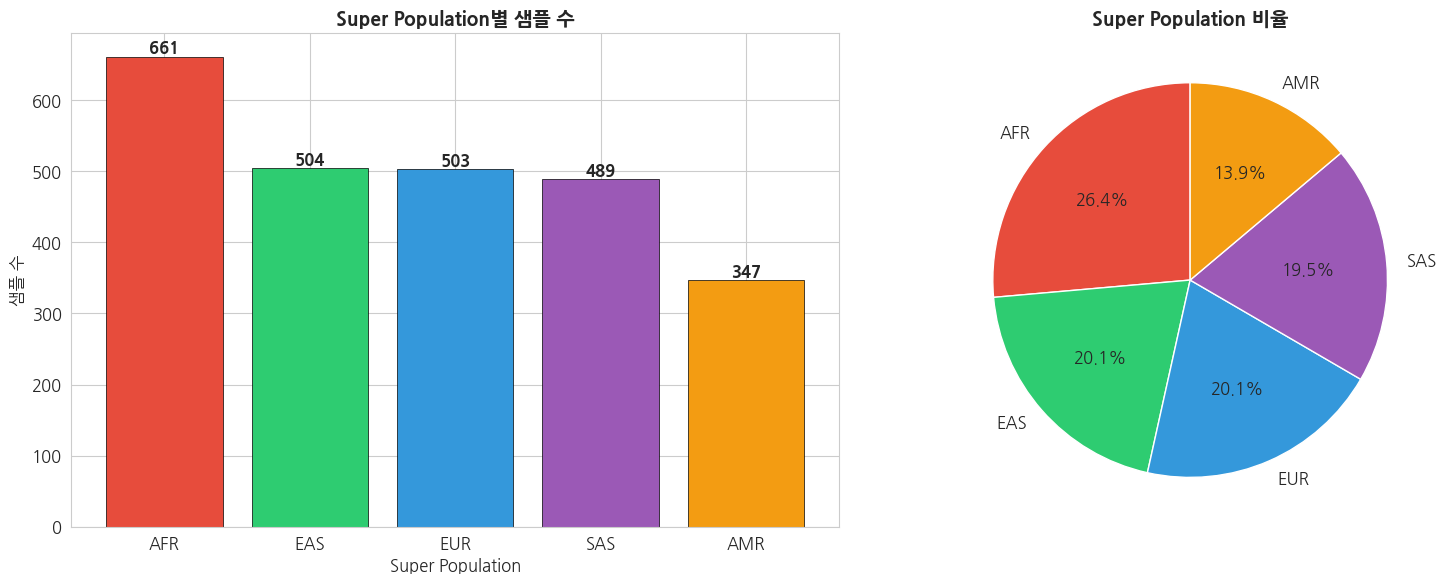

png

1.3 세부 Population 분포

python

# Population별 Super Population 매핑 테이블 생성
pop_superpop = panel.groupby(['super_pop', 'pop']).size().reset_index(name='count')
pop_superpop = pop_superpop.sort_values(['super_pop', 'count'], ascending=[True, False])

# 26개 Population 시각화
fig, ax = plt.subplots(figsize=(16, 8))

# Super Population별 색상 지정
bar_colors = [superpop_colors[row['super_pop']] for _, row in pop_superpop.iterrows()]

bars = ax.bar(range(len(pop_superpop)), pop_superpop['count'].values, color=bar_colors, edgecolor='black', linewidth=0.5)
ax.set_xticks(range(len(pop_superpop)))
ax.set_xticklabels(pop_superpop['pop'].values, rotation=45, ha='right')
ax.set_title('26개 Population별 샘플 수', fontsize=14, fontweight='bold')
ax.set_xlabel('Population')
ax.set_ylabel('샘플 수')

# 범례
from matplotlib.patches import Patch
legend_elements = [Patch(facecolor=superpop_colors[sp], edgecolor='black', label=sp) for sp in ['AFR', 'AMR', 'EAS', 'EUR', 'SAS']]
ax.legend(handles=legend_elements, title='Super Population', loc='upper right')

plt.tight_layout()
plt.show()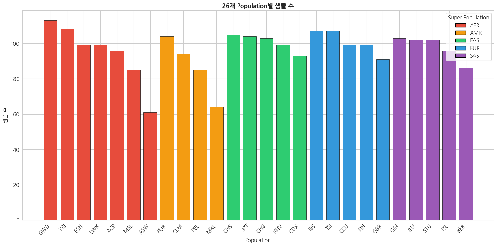

png

1.4 Pedigree (가계도) 데이터 로드

PED 파일은 가계 관계, 성별, 표현형 등의 정보를 포함합니다. PLINK에서 사용하는 표준 형식이기도 합니다.

python

# Pedigree 데이터 로드
ped_columns = [
    'Family_ID', 'Individual_ID', 'Paternal_ID', 'Maternal_ID',
    'Gender', 'Phenotype',
    'Population', 'Relationship', 'Siblings', 'Second_Order',
    'Third_Order', 'Other_Comments'
]

ped = pd.read_csv(
    f'{PHENOTYPE_DIR}/20130606_g1k.ped',
    sep='\t',
    header=0
)

print(f'Pedigree 데이터 샘플 수: {len(ped)}')
print(f'컬럼: {list(ped.columns)}')
print()
ped.head(10)

Pedigree 데이터 샘플 수: 3501
컬럼: ['Family ID', 'Individual ID', 'Paternal ID', 'Maternal ID', 'Gender', 'Phenotype', 'Population', 'Relationship', 'Siblings', 'Second Order', 'Third Order', 'Other Comments']

	Family ID	Individual ID	Paternal ID	Maternal ID	Gender	Population	Relationship
0	BB01	HG01879	0	0	1	ACB	father
1	BB01	HG01880	0	0	2	ACB	mother
2	BB01	HG01881	HG01879	HG01880	2	ACB	child
3	BB02	HG01882	0	0	1	ACB	father
4	BB02	HG01883	0	0	2	ACB	mother
5	BB02	HG01888	HG01882	HG01883	1	ACB	child
6	BB03	HG01884	HG01885	HG01956	2	ACB	child
7	BB03	HG01885	0	0	1	ACB	father
8	BB03	HG01956	0	0	2	ACB	mother
9	BB04	HG01886	0	0	2	ACB	mother

python

# PED 파일 주요 필드 설명
print('=== PED 파일 주요 필드 ===')
print('Family_ID      : 가족 ID')
print('Individual_ID  : 개인 ID (VCF 샘플명과 매칭)')
print('Paternal_ID    : 아버지 ID (0 = 정보없음)')
print('Maternal_ID    : 어머니 ID (0 = 정보없음)')
print('Gender         : 성별 (1=Male, 2=Female)')
print('Phenotype      : 표현형 (0=Missing, 1=Unaffected, 2=Affected)')
print()
print('=== Gender 분포 ===')
gender_col = [c for c in ped.columns if 'ender' in c.lower()][0]
print(ped[gender_col].value_counts())
print()
print('=== Relationship 분포 ===')
rel_col = [c for c in ped.columns if 'elation' in c.lower()][0]
print(ped[rel_col].value_counts())

=== PED 파일 주요 필드 ===
Family_ID      : 가족 ID
Individual_ID  : 개인 ID (VCF 샘플명과 매칭)
Paternal_ID    : 아버지 ID (0 = 정보없음)
Maternal_ID    : 어머니 ID (0 = 정보없음)
Gender         : 성별 (1=Male, 2=Female)
Phenotype      : 표현형 (0=Missing, 1=Unaffected, 2=Affected)

=== Gender 분포 ===
Gender
2    1761
1    1740
Name: count, dtype: int64

=== Relationship 분포 ===
Relationship
unrel                      1003
mother                      831
father                      816
child                       693
mat grandmother              31
mat grandfather              29
pat grandmother              28
pat grandfather              28
unrels                       14
Child2                        7
not father                    3
daughter                      1
father; child                 1
pat grandfather; father       1
mother; child                 1
pat grandmother; mother       1
mat grandfather; father       1
Child                         1
mat grandmother; mother       1
wife of child                 1
paternal father               1
paternal brother              1
child of 19672                1
child of 19740                1
child of 19752&3              1
child of 19764                1
husband of Child              1
maternal grandmother          1
paternal grandmother          1
Name: count, dtype: int64

1.5 샘플 상세 정보 (Excel)

python

# 샘플 상세 정보 로드
sample_info = pd.read_excel(
    f'{PHENOTYPE_DIR}/20130606_sample_info.xlsx',
    engine='openpyxl'
)

print(f'샘플 상세 정보 수: {len(sample_info)}')
print(f'컬럼 수: {len(sample_info.columns)}')
print(f'\n컬럼 목록:')
for i, col in enumerate(sample_info.columns, 1):
    print(f'  {i:2d}. {col}')
print()
sample_info.head()

샘플 상세 정보 수: 3500
컬럼 수: 15

컬럼 목록:
   1. Sample
   2. Family ID
   3. Population
   4. Population Description
   5. Gender
   6. Relationship
   7. Unexpected Parent/Child 
   8. Non Paternity
   9. Siblings
  10. Grandparents
  11. Avuncular
  12. Half Siblings
  13. Unknown Second Order
  14. Third Order
  15. Other Comments

	Sample	Family ID	Population	Population Description	Gender	Relationship	Unexpected Parent/Child	Non Paternity	Siblings	Grandparents	Avuncular	Half Siblings	Unknown Second Order	Third Order	Other Comments
0	HG00096	HG00096	GBR	British in England and Scotland	male	NaN	NaN	NaN	NaN	NaN	NaN	NaN	NaN	NaN	NaN
1	HG00097	HG00097	GBR	British in England and Scotland	female	NaN	NaN	NaN	NaN	NaN	NaN	NaN	NaN	NaN	NaN
2	HG00098	HG00098	GBR	British in England and Scotland	male	NaN	NaN	NaN	NaN	NaN	NaN	NaN	NaN	NaN	NaN
3	HG00099	HG00099	GBR	British in England and Scotland	female	NaN	NaN	NaN	NaN	NaN	NaN	NaN	NaN	NaN	NaN
4	HG00100	HG00100	GBR	British in England and Scotland	female	NaN	NaN	NaN	NaN	NaN	NaN	NaN	NaN	NaN	NaN

2. 임상 정보 통계 및 연관성 분석

2.1 데이터 통합

Panel 데이터와 Pedigree 데이터를 결합하여 종합적인 분석 데이터셋을 구축합니다.

python

# Panel 데이터와 Pedigree 데이터 병합
# panel의 'sample' 컬럼과 ped의 'Individual ID' 컬럼으로 매칭
ped_id_col = [c for c in ped.columns if 'ndividual' in c][0]

merged = panel.merge(
    ped,
    left_on='sample',
    right_on=ped_id_col,
    how='left'
)

print(f'병합 전 Panel 샘플 수: {len(panel)}')
print(f'병합 전 Pedigree 샘플 수: {len(ped)}')
print(f'병합 후 샘플 수: {len(merged)}')
print(f'\n병합 데이터 컬럼: {list(merged.columns)}')

병합 전 Panel 샘플 수: 2504
병합 전 Pedigree 샘플 수: 3501
병합 후 샘플 수: 2504

병합 데이터 컬럼: ['sample', 'pop', 'super_pop', 'gender', 'Unnamed: 4', 'Unnamed: 5', 'Family ID', 'Individual ID', 'Paternal ID', 'Maternal ID', 'Gender', 'Phenotype', 'Population', 'Relationship', 'Siblings', 'Second Order', 'Third Order', 'Other Comments']

2.2 성별(Gender) 분포 분석

python

# 성별 분포 - 전체 및 Super Population별
fig, axes = plt.subplots(1, 3, figsize=(18, 5))

# 전체 성별 분포
gender_counts = panel['gender'].value_counts()
axes[0].bar(gender_counts.index, gender_counts.values, color=['#3498db', '#e74c3c'], edgecolor='black')
axes[0].set_title('전체 성별 분포', fontsize=14, fontweight='bold')
axes[0].set_ylabel('샘플 수')
for i, (idx, val) in enumerate(gender_counts.items()):
    axes[0].text(i, val + 5, str(val), ha='center', fontweight='bold')

# Super Population별 성별 분포
gender_by_superpop = panel.groupby(['super_pop', 'gender']).size().unstack(fill_value=0)
gender_by_superpop.plot(kind='bar', ax=axes[1], color=['#e74c3c', '#3498db'], edgecolor='black', linewidth=0.5)
axes[1].set_title('Super Population별 성별 분포', fontsize=14, fontweight='bold')
axes[1].set_xlabel('Super Population')
axes[1].set_ylabel('샘플 수')
axes[1].legend(title='Gender')
axes[1].tick_params(axis='x', rotation=0)

# 성별 비율 (stacked)
gender_ratio = gender_by_superpop.div(gender_by_superpop.sum(axis=1), axis=0)
gender_ratio.plot(kind='bar', stacked=True, ax=axes[2], color=['#e74c3c', '#3498db'], edgecolor='black', linewidth=0.5)
axes[2].set_title('Super Population별 성별 비율', fontsize=14, fontweight='bold')
axes[2].set_xlabel('Super Population')
axes[2].set_ylabel('비율')
axes[2].legend(title='Gender')
axes[2].tick_params(axis='x', rotation=0)
axes[2].axhline(y=0.5, color='black', linestyle='--', alpha=0.5)

plt.tight_layout()
plt.show()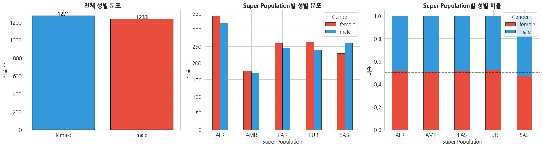

png

2.3 카이제곱 검정 (Chi-square Test)

Super Population과 성별 간에 통계적으로 유의미한 연관성이 있는지 확인합니다.

python

# Super Population × Gender 교차표
contingency_table = pd.crosstab(panel['super_pop'], panel['gender'])
print('=== 교차표 (Contingency Table) ===')
print(contingency_table)
print()

# 카이제곱 검정
chi2, p_value, dof, expected = stats.chi2_contingency(contingency_table)
print('=== 카이제곱 검정 결과 ===')
print(f'Chi-square statistic: {chi2:.4f}')
print(f'P-value: {p_value:.4f}')
print(f'Degrees of freedom: {dof}')
print()

if p_value < 0.05:
    print('→ p < 0.05: Super Population과 성별 간에 통계적으로 유의미한 연관성이 있습니다.')
else:
    print('→ p >= 0.05: Super Population과 성별 간에 통계적으로 유의미한 연관성이 없습니다.')
    print('  (각 Super Population에서 남녀 비율이 비슷하게 설계되었음을 의미합니다.)')

print()
print('=== 기대빈도 (Expected Frequencies) ===')
expected_df = pd.DataFrame(expected, index=contingency_table.index, columns=contingency_table.columns)
print(expected_df.round(1))

=== 교차표 (Contingency Table) ===
gender     female  male
super_pop              
AFR           342   319
AMR           177   170
EAS           260   244
EUR           263   240
SAS           229   260

=== 카이제곱 검정 결과 ===
Chi-square statistic: 3.8906
P-value: 0.4210
Degrees of freedom: 4

→ p >= 0.05: Super Population과 성별 간에 통계적으로 유의미한 연관성이 없습니다.
  (각 Super Population에서 남녀 비율이 비슷하게 설계되었음을 의미합니다.)

=== 기대빈도 (Expected Frequencies) ===
gender     female   male
super_pop               
AFR         335.5  325.5
AMR         176.1  170.9
EAS         255.8  248.2
EUR         255.3  247.7
SAS         248.2  240.8

2.4 Population별 샘플 크기 분석

python

# Population별 성별 구성 히트맵
pop_gender = pd.crosstab(panel['pop'], panel['gender'])
pop_gender['total'] = pop_gender.sum(axis=1)
pop_gender = pop_gender.sort_values('total', ascending=False)

# Super Population 정보 추가
pop_to_superpop = panel.drop_duplicates('pop').set_index('pop')['super_pop']

fig, ax = plt.subplots(figsize=(10, 10))
sns.heatmap(
    pop_gender[['female', 'male']],
    annot=True, fmt='d', cmap='YlOrRd',
    linewidths=0.5, ax=ax
)
ax.set_title('Population별 성별 분포 히트맵', fontsize=14, fontweight='bold')
ax.set_ylabel('Population')
ax.set_xlabel('Gender')

plt.tight_layout()
plt.show()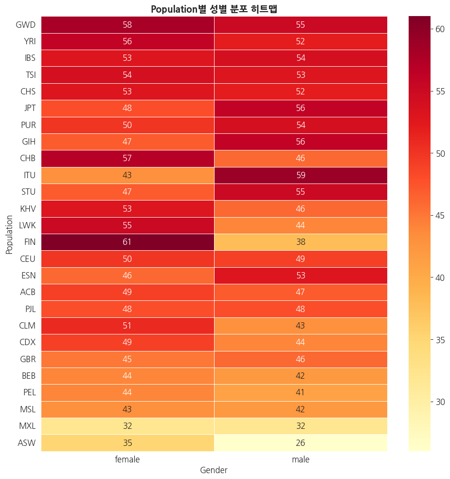

png

2.5 가계(Family) 구조 분석

python

# 가계 관계 분석
family_col = [c for c in ped.columns if 'amily' in c][0]
paternal_col = [c for c in ped.columns if 'aternal' in c][0]
maternal_col = [c for c in ped.columns if 'aternal' in c and 'M' in c[0]][0] if len([c for c in ped.columns if 'aternal' in c]) > 1 else [c for c in ped.columns if 'other' in c.lower() or 'maternal' in c.lower()][0]

# Relationship 분포
rel_col = [c for c in ped.columns if 'elation' in c.lower()][0]

fig, axes = plt.subplots(1, 2, figsize=(16, 6))

# Relationship 유형 분포
rel_counts = ped[rel_col].value_counts()
rel_counts.plot(kind='barh', ax=axes[0], color=sns.color_palette('Set2', len(rel_counts)), edgecolor='black')
axes[0].set_title('Relationship 유형별 분포', fontsize=14, fontweight='bold')
axes[0].set_xlabel('샘플 수')

# Trio 가족 식별 (부모 정보가 있는 샘플)
has_parents = ped[(ped[paternal_col] != '0') & (ped[paternal_col].notna())]
trio_count = len(has_parents)
unrelated_count = len(ped) - trio_count

axes[1].pie(
    [unrelated_count, trio_count],
    labels=['Unrelated', 'With Parents Info'],
    autopct='%1.1f%%',
    colors=['#3498db', '#e74c3c'],
    startangle=90,
    textprops={'fontsize': 12}
)
axes[1].set_title('부모 정보 유무', fontsize=14, fontweight='bold')

plt.tight_layout()
plt.show()

print(f'전체 샘플: {len(ped)}')
print(f'부모 정보 있는 샘플: {trio_count}')
print(f'Unrelated 샘플: {unrelated_count}')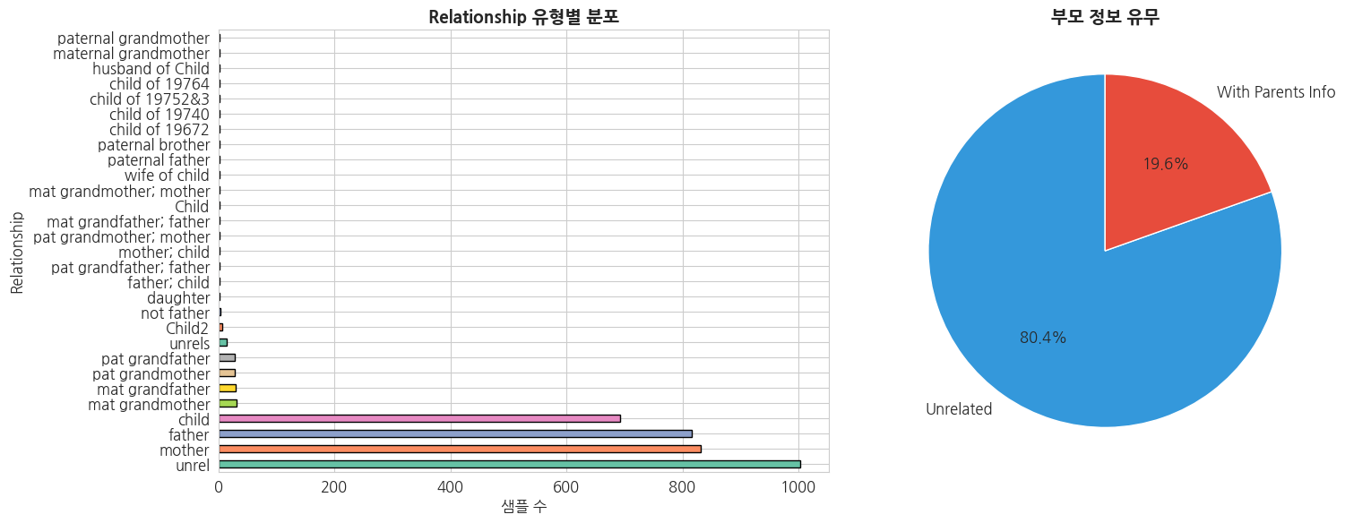

png

전체 샘플: 3501
부모 정보 있는 샘플: 685
Unrelated 샘플: 2816

2.6 Population 구조 요약 통계

python

# 포괄적 요약 통계 테이블 생성
summary_stats = panel.groupby('super_pop').agg(
    total_samples=('sample', 'count'),
    n_populations=('pop', 'nunique'),
    n_male=('gender', lambda x: (x == 'male').sum()),
    n_female=('gender', lambda x: (x == 'female').sum())
).reset_index()

summary_stats['male_ratio'] = (summary_stats['n_male'] / summary_stats['total_samples'] * 100).round(1)
summary_stats['female_ratio'] = (summary_stats['n_female'] / summary_stats['total_samples'] * 100).round(1)

# Super Population 설명 추가
sp_description = {
    'AFR': 'African',
    'AMR': 'Ad Mixed American',
    'EAS': 'East Asian',
    'EUR': 'European',
    'SAS': 'South Asian'
}
summary_stats['description'] = summary_stats['super_pop'].map(sp_description)

print('=== Super Population별 요약 통계 ===')
display_cols = ['super_pop', 'description', 'total_samples', 'n_populations', 'n_male', 'n_female', 'male_ratio', 'female_ratio']
summary_stats[display_cols]

=== Super Population별 요약 통계 ===

	super_pop	description	total_samples	n_populations	n_male	n_female	male_ratio	female_ratio
0	AFR	African	661	7	319	342	48.3	51.7
1	AMR	Ad Mixed American	347	4	170	177	49.0	51.0
2	EAS	East Asian	504	5	244	260	48.4	51.6
3	EUR	European	503	5	240	263	47.7	52.3
4	SAS	South Asian	489	5	260	229	53.2	46.8

3. 유전변이(VCF)-임상 표현형 통합 분석을 위한 전처리

VCF 파일과 임상 표현형 데이터를 결합하기 위한 전처리를 수행합니다.

3.1 VCF 파일 샘플 목록 추출

python

import subprocess

# VCF 파일에서 샘플 목록 추출 (bcftools 사용)
vcf_path = f'{INDIVIDUAL_DIR}/ALL.chr22.phase3_shapeit2_mvncall_integrated_v5b.20130502.genotypes.vcf.gz'

result = subprocess.run(
    ['bcftools', 'query', '-l', vcf_path],
    capture_output=True, text=True
)

vcf_samples = result.stdout.strip().split('\n')
print(f'VCF 파일 내 샘플 수: {len(vcf_samples)}')
print(f'처음 10개 샘플: {vcf_samples[:10]}')

VCF 파일 내 샘플 수: 2504
처음 10개 샘플: ['HG00096', 'HG00097', 'HG00099', 'HG00100', 'HG00101', 'HG00102', 'HG00103', 'HG00105', 'HG00106', 'HG00107']

python

# Panel 데이터와 VCF 샘플 간 매칭 확인
panel_samples = set(panel['sample'].values)
vcf_sample_set = set(vcf_samples)

common_samples = panel_samples & vcf_sample_set
only_panel = panel_samples - vcf_sample_set
only_vcf = vcf_sample_set - panel_samples

print(f'Panel에만 있는 샘플: {len(only_panel)}')
print(f'VCF에만 있는 샘플: {len(only_vcf)}')
print(f'공통 샘플: {len(common_samples)}')
print(f'\n→ Panel과 VCF의 샘플이 완전히 일치합니다.' if len(only_panel) == 0 and len(only_vcf) == 0 else f'\n→ 불일치 샘플이 있습니다.')

Panel에만 있는 샘플: 0
VCF에만 있는 샘플: 0
공통 샘플: 2504

→ Panel과 VCF의 샘플이 완전히 일치합니다.

3.2 분석용 통합 데이터셋 구축

VCF의 샘플 순서와 임상 정보를 정확히 매칭한 통합 데이터셋을 생성합니다.

python

# VCF 샘플 순서에 맞춰 panel 정보 정렬
vcf_sample_df = pd.DataFrame({'sample': vcf_samples, 'vcf_order': range(len(vcf_samples))})

# 통합 데이터셋 생성
integrated = vcf_sample_df.merge(panel, on='sample', how='left')

print(f'통합 데이터셋 크기: {integrated.shape}')
print(f'결측치 확인:')
print(integrated.isnull().sum())
print()
integrated.head(10)

통합 데이터셋 크기: (2504, 7)
결측치 확인:
sample           0
vcf_order        0
pop              0
super_pop        0
gender           0
Unnamed: 4    2504
Unnamed: 5    2504
dtype: int64

	sample	vcf_order	pop	super_pop	gender	Unnamed: 4	Unnamed: 5
0	HG00096	0	GBR	EUR	male	NaN	NaN
1	HG00097	1	GBR	EUR	female	NaN	NaN
2	HG00099	2	GBR	EUR	female	NaN	NaN
3	HG00100	3	GBR	EUR	female	NaN	NaN
4	HG00101	4	GBR	EUR	male	NaN	NaN
5	HG00102	5	GBR	EUR	female	NaN	NaN
6	HG00103	6	GBR	EUR	male	NaN	NaN
7	HG00105	7	GBR	EUR	male	NaN	NaN
8	HG00106	8	GBR	EUR	female	NaN	NaN
9	HG00107	9	GBR	EUR	male	NaN	NaN

3.3 분석 대상 서브셋 생성

특정 분석 목적에 맞는 서브셋을 미리 정의합니다.

python

# EAS (동아시아) 서브셋 - 한국인 관련 분석에 활용
eas_samples = integrated[integrated['super_pop'] == 'EAS']
print(f'=== EAS (동아시아) 서브셋 ===')
print(f'샘플 수: {len(eas_samples)}')
print(f'포함 Population: {eas_samples["pop"].unique()}')
print(f'  - CDX: Chinese Dai in Xishuangbanna')
print(f'  - CHB: Han Chinese in Beijing')
print(f'  - CHS: Southern Han Chinese')
print(f'  - JPT: Japanese in Tokyo')
print(f'  - KHV: Kinh in Ho Chi Minh City')
print()

# Unrelated 샘플만 추출 (GWAS 분석용)
# Pedigree에서 관계 정보 확인하여 unrelated 샘플 필터링
ped_id_col = [c for c in ped.columns if 'ndividual' in c][0]
paternal_col = [c for c in ped.columns if 'aternal' in c][0]

unrelated_ids = ped[ped[paternal_col] == '0'][ped_id_col].values
unrelated_samples = integrated[integrated['sample'].isin(unrelated_ids)]
print(f'=== Unrelated 샘플 서브셋 (GWAS용) ===')
print(f'전체: {len(integrated)} → Unrelated: {len(unrelated_samples)}')

=== EAS (동아시아) 서브셋 ===
샘플 수: 504
포함 Population: ['CHS' 'CDX' 'KHV' 'CHB' 'JPT']
  - CDX: Chinese Dai in Xishuangbanna
  - CHB: Han Chinese in Beijing
  - CHS: Southern Han Chinese
  - JPT: Japanese in Tokyo
  - KHV: Kinh in Ho Chi Minh City

=== Unrelated 샘플 서브셋 (GWAS용) ===
전체: 2504 → Unrelated: 2495

3.4 개인 샘플 VCF에서 기본 변이 통계 미리보기

1명의 샘플을 선택하여 VCF에서 기본적인 변이 정보를 추출합니다. (2강에서 상세 분석 예정)

python

# 샘플 1명 선택 (EAS - JPT 일본인 샘플)
target_sample = eas_samples[eas_samples['pop'] == 'JPT']['sample'].values[0]
print(f'선택 샘플: {target_sample}')
print(f'Population: JPT (Japanese in Tokyo)')
print(f'Super Population: EAS (East Asian)')
print()

# bcftools로 해당 샘플의 변이 수 확인 (chr22 기준)
result = subprocess.run(
    ['bcftools', 'view', '-s', target_sample, '--min-ac', '1', '-H', vcf_path],
    capture_output=True, text=True
)

variant_lines = result.stdout.strip().split('\n')
n_variants = len([l for l in variant_lines if l.strip()])
print(f'{target_sample}의 chr22 변이 수: {n_variants:,}')

선택 샘플: NA18939
Population: JPT (Japanese in Tokyo)
Super Population: EAS (East Asian)

NA18939의 chr22 변이 수: 56,754

python

# 해당 샘플의 변이 타입 미리보기 (처음 1000개만)
result = subprocess.run(
    ['bcftools', 'view', '-s', target_sample, '--min-ac', '1', vcf_path],
    capture_output=True, text=True
)

# 변이 타입 분류
snp_count = 0
indel_count = 0
other_count = 0

for line in variant_lines[:5000]:
    if not line.strip() or line.startswith('#'):
        continue
    fields = line.split('\t')
    if len(fields) < 5:
        continue
    ref = fields[3]
    alts = fields[4].split(',')
    is_snp = all(len(alt) == 1 and len(ref) == 1 for alt in alts)
    if is_snp:
        snp_count += 1
    else:
        indel_count += 1

print(f'=== {target_sample} chr22 변이 타입 미리보기 (처음 5000개) ===')
print(f'SNP: {snp_count:,}')
print(f'INDEL: {indel_count:,}')
print(f'\n→ 2강에서 VCF 구조 및 변이 타입에 대해 상세히 분석합니다.')

=== NA18939 chr22 변이 타입 미리보기 (처음 5000개) ===
SNP: 4,354
INDEL: 646

→ 2강에서 VCF 구조 및 변이 타입에 대해 상세히 분석합니다.

3.5 전처리된 데이터 저장

후속 강의에서 사용할 수 있도록 통합 데이터를 저장합니다.

python

# 통합 임상 데이터 저장
output_path = f'{DATA_DIR}/phenotype/integrated_sample_info.tsv'
integrated.to_csv(output_path, sep='\t', index=False)
print(f'통합 데이터 저장 완료: {output_path}')
print(f'  - 샘플 수: {len(integrated)}')
print(f'  - 컬럼: {list(integrated.columns)}')

# EAS 서브셋 저장
eas_output = f'{DATA_DIR}/phenotype/eas_sample_info.tsv'
eas_samples.to_csv(eas_output, sep='\t', index=False)
print(f'\nEAS 서브셋 저장 완료: {eas_output}')
print(f'  - 샘플 수: {len(eas_samples)}')

# Unrelated 샘플 목록 저장 (GWAS용)
unrelated_output = f'{DATA_DIR}/phenotype/unrelated_samples.txt'
unrelated_samples[['sample']].to_csv(unrelated_output, sep='\t', index=False, header=False)
print(f'\nUnrelated 샘플 목록 저장 완료: {unrelated_output}')
print(f'  - 샘플 수: {len(unrelated_samples)}')

통합 데이터 저장 완료: /tier4/DSC/jheepark/bbp-wgs-data/phenotype/integrated_sample_info.tsv
  - 샘플 수: 2504
  - 컬럼: ['sample', 'vcf_order', 'pop', 'super_pop', 'gender', 'Unnamed: 4', 'Unnamed: 5']

EAS 서브셋 저장 완료: /tier4/DSC/jheepark/bbp-wgs-data/phenotype/eas_sample_info.tsv
  - 샘플 수: 504

Unrelated 샘플 목록 저장 완료: /tier4/DSC/jheepark/bbp-wgs-data/phenotype/unrelated_samples.txt
  - 샘플 수: 2495

4. 요약 및 다음 강의 안내

이번 강의 요약

항목	내용
데이터 소스	1000 Genomes Project Phase 3
전체 샘플	2,504명
Super Population	5개 (AFR, AMR, EAS, EUR, SAS)
세부 Population	26개
주요 분석	인구집단 분포, 성별 연관성(χ²), 가계 구조
전처리 산출물	통합 데이터셋, EAS 서브셋, Unrelated 샘플 목록

핵심 포인트

WGS 분석 전 임상/표현형 데이터의 구조를 이해하는 것이 중요합니다.
인구집단 구성, 성별 분포, 가계 관계 등은 후속 유전 분석의 교란 요인이 될 수 있습니다.
VCF 데이터와 임상 정보의 샘플 ID 매칭을 반드시 확인해야 합니다.
분석 목적에 따라 적절한 서브셋 (예: Unrelated 샘플) 을 선별하는 것이 필요합니다.

다음 강의 예고

2강: VCF 기초 통계 분석

VCF 파일의 주요 컬럼 확인 및 통계 지표 계산
SNP·INDEL 등 변이 타입 분포 시각화
Mutation Profile 기반 변이 특성 요약
필터링 조건별 변이 수 비교 분석

1강: 표현형 기반 임상 데이터 기초 통계 분석 ​

BBP WGS 분석 튜토리얼 ​

학습 목표 ​

사용 데이터 ​

산출물 (본 강의에서 생성) ​

사용 도구 ​

0. 환경 설정 ​

1. 표현형 기반 임상 데이터 구조 이해 ​

1.1 샘플 패널 데이터 로드 ​

1.2 Super Population (대륙 그룹) 이해 ​

1.3 세부 Population 분포 ​

1.4 Pedigree (가계도) 데이터 로드 ​

1.5 샘플 상세 정보 (Excel) ​

2. 임상 정보 통계 및 연관성 분석 ​

2.1 데이터 통합 ​

2.2 성별(Gender) 분포 분석 ​

2.3 카이제곱 검정 (Chi-square Test) ​

2.4 Population별 샘플 크기 분석 ​

2.5 가계(Family) 구조 분석 ​

2.6 Population 구조 요약 통계 ​

3. 유전변이(VCF)-임상 표현형 통합 분석을 위한 전처리 ​

3.1 VCF 파일 샘플 목록 추출 ​

3.2 분석용 통합 데이터셋 구축 ​

3.3 분석 대상 서브셋 생성 ​

3.4 개인 샘플 VCF에서 기본 변이 통계 미리보기 ​

3.5 전처리된 데이터 저장 ​

4. 요약 및 다음 강의 안내 ​

이번 강의 요약 ​

핵심 포인트 ​

다음 강의 예고 ​

1강: 표현형 기반 임상 데이터 기초 통계 분석

BBP WGS 분석 튜토리얼

학습 목표

사용 데이터

산출물 (본 강의에서 생성)

사용 도구

0. 환경 설정

1. 표현형 기반 임상 데이터 구조 이해

1.1 샘플 패널 데이터 로드

1.2 Super Population (대륙 그룹) 이해

1.3 세부 Population 분포

1.4 Pedigree (가계도) 데이터 로드

1.5 샘플 상세 정보 (Excel)

2. 임상 정보 통계 및 연관성 분석

2.1 데이터 통합

2.2 성별(Gender) 분포 분석

2.3 카이제곱 검정 (Chi-square Test)

2.4 Population별 샘플 크기 분석

2.5 가계(Family) 구조 분석

2.6 Population 구조 요약 통계

3. 유전변이(VCF)-임상 표현형 통합 분석을 위한 전처리

3.1 VCF 파일 샘플 목록 추출

3.2 분석용 통합 데이터셋 구축

3.3 분석 대상 서브셋 생성

3.4 개인 샘플 VCF에서 기본 변이 통계 미리보기

3.5 전처리된 데이터 저장

4. 요약 및 다음 강의 안내

이번 강의 요약

핵심 포인트

다음 강의 예고