2강: VCF 기초 통계 분석

BBP WGS 분석 튜토리얼

학습 목표

VCF 파일 주요 컬럼 확인 및 통계 지표 계산 - VCF 형식 이해 및 기본 통계 산출
SNP·INDEL 등 변이 타입 분포 시각화 - 변이 유형별 분포 분석
Mutation Profile 기반 변이 특성 요약 - SNP의 염기 치환 패턴 분석
필터링 조건별 변이 수 비교 분석 - Quality, MAF 등 필터링 기준 비교

사용 데이터

데이터 루트: /tier4/DSC/jheepark/bbp-wgs-data/

데이터	경로	설명
1000 Genomes chr22 VCF	`individual/ALL.chr22.phase3_shapeit2_mvncall_integrated_v5b.20130502.genotypes.vcf.gz`	2,504 샘플 joint VCF, GRCh37
통합 샘플 정보	`phenotype/integrated_sample_info.tsv`	1강에서 생성한 Panel + Pedigree 병합 데이터 (Super Population별 대표 샘플 선정용)

산출물 (본 강의에서 생성)

파일	경로	설명
vcftools 통계 파일	`individual/chr22_stats.frq`	변이별 allele frequency
vcftools 통계 파일	`individual/chr22_stats.ldepth.mean`	Site 별 mean depth
vcftools 통계 파일	`individual/chr22_stats.lmiss`	Site 별 missingness

사용 도구

bcftools, vcftools
Python: cyvcf2, pandas, numpy, matplotlib, seaborn

0. 환경 설정

python

import pandas as pd
import numpy as np
import matplotlib.pyplot as plt
import seaborn as sns
from cyvcf2 import VCF
from collections import Counter, defaultdict
from matplotlib import font_manager, rc
import subprocess
import warnings
warnings.filterwarnings('ignore')

# 시각화 설정 (seaborn 스타일을 먼저 설정해야 한글 폰트가 덮어씌워지지 않음)
sns.set_style('whitegrid')
sns.set_palette('Set2')

# 한글 폰트 설정 (seaborn 설정 이후에 적용)
font_path = '/usr/share/fonts/truetype/nanum/NanumGothic.ttf'
font_manager.fontManager.addfont(font_path)
rc('font', family='NanumGothic')
plt.rcParams['axes.unicode_minus'] = False  # 마이너스 기호 깨짐 방지
plt.rcParams['figure.figsize'] = (12, 6)
plt.rcParams['font.size'] = 12

# 데이터 경로
DATA_DIR = '/tier4/DSC/jheepark/bbp-wgs-data'
VCF_PATH = f'{DATA_DIR}/individual/ALL.chr22.phase3_shapeit2_mvncall_integrated_v5b.20130502.genotypes.vcf.gz'

print('환경 설정 완료!')
print(f'VCF 파일: {VCF_PATH}')

환경 설정 완료!
VCF 파일: /tier4/DSC/jheepark/bbp-wgs-data/individual/ALL.chr22.phase3_shapeit2_mvncall_integrated_v5b.20130502.genotypes.vcf.gz

1. VCF 파일 구조 이해

VCF (Variant Call Format) 파일이란?

VCF는 유전체 변이(variant) 정보를 저장하는 표준 형식입니다.

VCF 파일 구성

## 헤더 (메타 정보)
##fileformat=VCFv4.1
##INFO=<ID=AF,Number=A,Type=Float,Description="Allele Frequency">
##FORMAT=<ID=GT,Number=1,Type=String,Description="Genotype">

# 컬럼 헤더
#CHROM  POS     ID      REF     ALT     QUAL    FILTER  INFO    FORMAT  SAMPLE1 SAMPLE2 ...

# 데이터 행
22      16050075  .     A       G       100     PASS    AF=0.5  GT      0|0     0|1     ...

1.1 VCF 헤더 확인

python

# VCF 헤더 확인 (bcftools)
result = subprocess.run(
    ['bcftools', 'view', '-h', VCF_PATH],
    capture_output=True, text=True
)

header_lines = result.stdout.strip().split('\n')
print(f'헤더 라인 수: {len(header_lines)}')
print()

# 메타 정보 유형별 분류
meta_types = Counter()
for line in header_lines:
    if line.startswith('##'):
        key = line.split('=')[0].replace('##', '')
        meta_types[key] += 1

print('=== 헤더 메타 정보 유형 ===')
for key, count in meta_types.most_common():
    print(f'  {key}: {count}개')

헤더 라인 수: 255

=== 헤더 메타 정보 유형 ===
  ALT: 133개
  contig: 86개
  INFO: 27개
  fileformat: 1개
  FILTER: 1개
  fileDate: 1개
  reference: 1개
  source: 1개
  FORMAT: 1개
  bcftools_viewVersion: 1개
  bcftools_viewCommand: 1개

python

# INFO 필드 정의 확인
print('=== 주요 INFO 필드 ===')
for line in header_lines:
    if line.startswith('##INFO'):
        print(line)

=== 주요 INFO 필드 ===
##INFO=<ID=CIEND,Number=2,Type=Integer,Description="Confidence interval around END for imprecise variants">
##INFO=<ID=CIPOS,Number=2,Type=Integer,Description="Confidence interval around POS for imprecise variants">
##INFO=<ID=CS,Number=1,Type=String,Description="Source call set.">
##INFO=<ID=END,Number=1,Type=Integer,Description="End coordinate of this variant">
##INFO=<ID=IMPRECISE,Number=0,Type=Flag,Description="Imprecise structural variation">
##INFO=<ID=MC,Number=.,Type=String,Description="Merged calls.">
##INFO=<ID=MEINFO,Number=4,Type=String,Description="Mobile element info of the form NAME,START,END<POLARITY; If there is only 5' OR 3' support for this call, will be NULL NULL for START and END">
##INFO=<ID=MEND,Number=1,Type=Integer,Description="Mitochondrial end coordinate of inserted sequence">
##INFO=<ID=MLEN,Number=1,Type=Integer,Description="Estimated length of mitochondrial insert">
##INFO=<ID=MSTART,Number=1,Type=Integer,Description="Mitochondrial start coordinate of inserted sequence">
##INFO=<ID=SVLEN,Number=.,Type=Integer,Description="SV length. It is only calculated for structural variation MEIs. For other types of SVs; one may calculate the SV length by INFO:END-START+1, or by finding the difference between lengthes of REF and ALT alleles">
##INFO=<ID=SVTYPE,Number=1,Type=String,Description="Type of structural variant">
##INFO=<ID=TSD,Number=1,Type=String,Description="Precise Target Site Duplication for bases, if unknown, value will be NULL">
##INFO=<ID=AC,Number=A,Type=Integer,Description="Total number of alternate alleles in called genotypes">
##INFO=<ID=AF,Number=A,Type=Float,Description="Estimated allele frequency in the range (0,1)">
##INFO=<ID=NS,Number=1,Type=Integer,Description="Number of samples with data">
##INFO=<ID=AN,Number=1,Type=Integer,Description="Total number of alleles in called genotypes">
##INFO=<ID=EAS_AF,Number=A,Type=Float,Description="Allele frequency in the EAS populations calculated from AC and AN, in the range (0,1)">
##INFO=<ID=EUR_AF,Number=A,Type=Float,Description="Allele frequency in the EUR populations calculated from AC and AN, in the range (0,1)">
##INFO=<ID=AFR_AF,Number=A,Type=Float,Description="Allele frequency in the AFR populations calculated from AC and AN, in the range (0,1)">
##INFO=<ID=AMR_AF,Number=A,Type=Float,Description="Allele frequency in the AMR populations calculated from AC and AN, in the range (0,1)">
##INFO=<ID=SAS_AF,Number=A,Type=Float,Description="Allele frequency in the SAS populations calculated from AC and AN, in the range (0,1)">
##INFO=<ID=DP,Number=1,Type=Integer,Description="Total read depth; only low coverage data were counted towards the DP, exome data were not used">
##INFO=<ID=AA,Number=1,Type=String,Description="Ancestral Allele. Format: AA|REF|ALT|IndelType. AA: Ancestral allele, REF:Reference Allele, ALT:Alternate Allele, IndelType:Type of Indel (REF, ALT and IndelType are only defined for indels)">
##INFO=<ID=VT,Number=.,Type=String,Description="indicates what type of variant the line represents">
##INFO=<ID=EX_TARGET,Number=0,Type=Flag,Description="indicates whether a variant is within the exon pull down target boundaries">
##INFO=<ID=MULTI_ALLELIC,Number=0,Type=Flag,Description="indicates whether a site is multi-allelic">

python

# FORMAT 필드 정의 확인
print('=== FORMAT 필드 ===')
for line in header_lines:
    if line.startswith('##FORMAT'):
        print(line)

=== FORMAT 필드 ===
##FORMAT=<ID=GT,Number=1,Type=String,Description="Genotype">

1.2 VCF 주요 8개 고정 컬럼

컬럼	설명	예시
CHROM	염색체 번호	22
POS	변이 위치 (1-based)	16050075
ID	변이 식별자 (rsID)	rs587697622
REF	Reference allele	A
ALT	Alternative allele(s)	G
QUAL	변이 품질 점수	100
FILTER	필터 상태	PASS
INFO	변이 주석 정보	AF=0.5;AC=2504

python

# VCF 데이터 첫 10행 확인
result = subprocess.run(
    ['bcftools', 'view', '-H', VCF_PATH],
    capture_output=True, text=True
)

lines = result.stdout.strip().split('\n')[:10]
print('=== VCF 데이터 (처음 10행, 주요 컬럼만 표시) ===')
print(f'{"CHROM":>6} {"POS":>12} {"ID":>15} {"REF":>5} {"ALT":>5} {"QUAL":>6} {"FILTER":>8}')
print('-' * 65)
for line in lines:
    fields = line.split('\t')
    print(f'{fields[0]:>6} {fields[1]:>12} {fields[2]:>15} {fields[3]:>5} {fields[4]:>5} {fields[5]:>6} {fields[6]:>8}')

=== VCF 데이터 (처음 10행, 주요 컬럼만 표시) ===
 CHROM          POS              ID   REF   ALT   QUAL   FILTER
-----------------------------------------------------------------
    22     16050075               .     A     G    100     PASS
    22     16050115               .     G     A    100     PASS
    22     16050213               .     C     T    100     PASS
    22     16050319               .     C     T    100     PASS
    22     16050527               .     C     A    100     PASS
    22     16050568               .     C     A    100     PASS
    22     16050607               .     G     A    100     PASS
    22     16050627               .     G     T    100     PASS
    22     16050646               .     G     T    100     PASS
    22     16050654               .     A <CN0>,<CN2>,<CN3>,<CN4>    100     PASS

1.3 bcftools stats로 기본 통계 확인

python

# bcftools stats 실행
result = subprocess.run(
    ['bcftools', 'stats', VCF_PATH],
    capture_output=True, text=True
)

# SN (Summary Numbers) 파싱
print('=== bcftools stats - Summary Numbers ===')
for line in result.stdout.split('\n'):
    if line.startswith('SN'):
        print(line)

=== bcftools stats - Summary Numbers ===
SN	0	number of samples:	2504
SN	0	number of records:	1103547
SN	0	number of no-ALTs:	0
SN	0	number of SNPs:	1060388
SN	0	number of MNPs:	0
SN	0	number of indels:	43230
SN	0	number of others:	801
SN	0	number of multiallelic sites:	6348
SN	0	number of multiallelic SNP sites:	4063

python

# Ts/Tv (Transition/Transversion) 비율
print('=== Transition/Transversion 비율 ===')
for line in result.stdout.split('\n'):
    if line.startswith('TSTV'):
        fields = line.split('\t')
        print(f'Transitions (Ts): {fields[2]}')
        print(f'Transversions (Tv): {fields[3]}')
        print(f'Ts/Tv ratio: {fields[4]}')
        print()
        print('※ Ts/Tv 비율 해석:')
        print('  - WGS 전체: ~2.0-2.1 (예상값)')
        print('  - Exome: ~2.8-3.0')
        print('  - 1.0 미만: 데이터 품질 문제 가능성')

=== Transition/Transversion 비율 ===
Transitions (Ts): 750034
Transversions (Tv): 314468
Ts/Tv ratio: 2.39

※ Ts/Tv 비율 해석:
  - WGS 전체: ~2.0-2.1 (예상값)
  - Exome: ~2.8-3.0
  - 1.0 미만: 데이터 품질 문제 가능성

2. SNP·INDEL 등 변이 타입 분포 시각화

2.1 cyvcf2를 이용한 변이 타입 분류

python

# cyvcf2로 VCF 로드 및 변이 타입 분류
vcf = VCF(VCF_PATH)

variant_types = Counter()  # SNP, INDEL, MNP, etc.
variant_subtypes = Counter()  # insertion, deletion, ts, tv
alt_allele_counts = Counter()  # multi-allelic 여부
qual_scores = []
positions = []
af_values = []

# 변이 정보 수집
for i, variant in enumerate(vcf):
    # 변이 타입 분류
    if variant.is_snp:
        variant_types['SNP'] += 1
    elif variant.is_indel:
        variant_types['INDEL'] += 1
        # Insertion vs Deletion
        for alt in variant.ALT:
            if len(alt) > len(variant.REF):
                variant_subtypes['Insertion'] += 1
            elif len(alt) < len(variant.REF):
                variant_subtypes['Deletion'] += 1
    else:
        variant_types['Other'] += 1
    
    # Alt allele 수
    alt_allele_counts[len(variant.ALT)] += 1
    
    # 위치 정보
    positions.append(variant.POS)
    
    # Allele Frequency
    af = variant.INFO.get('AF')
    if af is not None:
        if isinstance(af, (tuple, list)):
            af_values.append(af[0])
        else:
            af_values.append(af)

vcf.close()

total_variants = sum(variant_types.values())
print(f'=== 전체 변이 통계 (chr22) ===')
print(f'총 변이 수: {total_variants:,}')
print()
for vtype, count in variant_types.most_common():
    print(f'  {vtype}: {count:,} ({count/total_variants*100:.1f}%)')

=== 전체 변이 통계 (chr22) ===
총 변이 수: 1,103,547

  SNP: 1,059,517 (96.0%)
  INDEL: 43,248 (3.9%)
  Other: 782 (0.1%)

python

# 변이 타입 분포 시각화
fig, axes = plt.subplots(1, 3, figsize=(18, 5))

# 1. 변이 타입 (SNP vs INDEL)
types = list(variant_types.keys())
counts = list(variant_types.values())
colors = ['#3498db', '#e74c3c', '#95a5a6']
bars = axes[0].bar(types, counts, color=colors[:len(types)], edgecolor='black', linewidth=0.5)
axes[0].set_title('변이 타입 분포', fontsize=14, fontweight='bold')
axes[0].set_ylabel('변이 수')
for bar, count in zip(bars, counts):
    axes[0].text(bar.get_x() + bar.get_width()/2, bar.get_height() + total_variants*0.01,
                f'{count:,}\n({count/total_variants*100:.1f}%)',
                ha='center', fontweight='bold', fontsize=10)

# 2. INDEL 세부 (Insertion vs Deletion)
if variant_subtypes:
    sub_types = list(variant_subtypes.keys())
    sub_counts = list(variant_subtypes.values())
    axes[1].bar(sub_types, sub_counts, color=['#2ecc71', '#e67e22'], edgecolor='black', linewidth=0.5)
    axes[1].set_title('INDEL 세부 분류', fontsize=14, fontweight='bold')
    axes[1].set_ylabel('변이 수')
    for i, (st, sc) in enumerate(zip(sub_types, sub_counts)):
        axes[1].text(i, sc + max(sub_counts)*0.01, f'{sc:,}', ha='center', fontweight='bold')

# 3. Multi-allelic 분포
allele_types = sorted(alt_allele_counts.keys())
allele_counts = [alt_allele_counts[k] for k in allele_types]
labels = [f'{k} ALT' for k in allele_types]
axes[2].bar(labels, allele_counts, color='#9b59b6', edgecolor='black', linewidth=0.5)
axes[2].set_title('ALT Allele 수 분포', fontsize=14, fontweight='bold')
axes[2].set_ylabel('변이 수')
axes[2].set_yscale('log')
for i, (l, c) in enumerate(zip(labels, allele_counts)):
    axes[2].text(i, c * 1.2, f'{c:,}', ha='center', fontweight='bold', fontsize=9)

plt.tight_layout()
plt.show()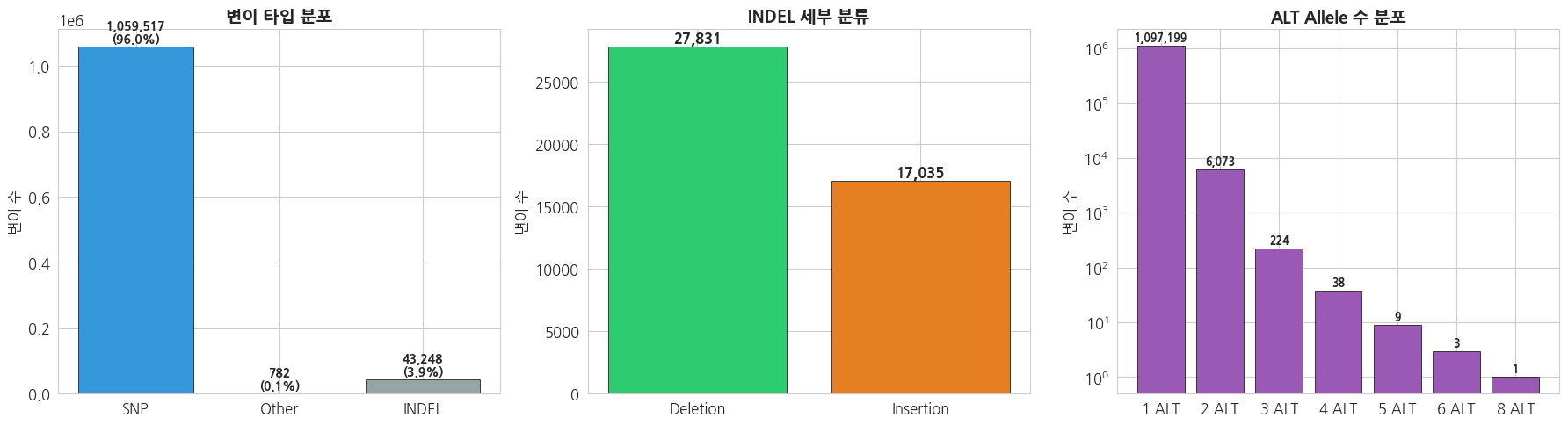

png

2.2 Allele Frequency (AF) 분포

python

# Allele Frequency 분포 시각화
af_array = np.array(af_values)

fig, axes = plt.subplots(1, 3, figsize=(18, 5))

# 1. AF 전체 분포 (히스토그램)
axes[0].hist(af_array, bins=50, color='#3498db', edgecolor='black', linewidth=0.3, alpha=0.8)
axes[0].set_title('Allele Frequency 분포', fontsize=14, fontweight='bold')
axes[0].set_xlabel('Allele Frequency (AF)')
axes[0].set_ylabel('변이 수')
axes[0].set_yscale('log')

# 2. AF 구간별 분류
af_categories = {
    'Rare\n(AF<0.01)': np.sum(af_array < 0.01),
    'Low freq\n(0.01-0.05)': np.sum((af_array >= 0.01) & (af_array < 0.05)),
    'Common\n(AF≥0.05)': np.sum(af_array >= 0.05)
}
cat_names = list(af_categories.keys())
cat_counts = list(af_categories.values())
bars = axes[1].bar(cat_names, cat_counts, color=['#e74c3c', '#f39c12', '#2ecc71'], edgecolor='black')
axes[1].set_title('변이 빈도 분류', fontsize=14, fontweight='bold')
axes[1].set_ylabel('변이 수')
for bar, count in zip(bars, cat_counts):
    axes[1].text(bar.get_x() + bar.get_width()/2, bar.get_height() + max(cat_counts)*0.01,
                f'{count:,}\n({count/len(af_array)*100:.1f}%)', ha='center', fontweight='bold', fontsize=10)

# 3. Rare variant AF 확대 (AF < 0.05)
rare_af = af_array[af_array < 0.05]
axes[2].hist(rare_af, bins=50, color='#e74c3c', edgecolor='black', linewidth=0.3, alpha=0.8)
axes[2].set_title('Rare Variant AF 분포 (AF < 0.05)', fontsize=14, fontweight='bold')
axes[2].set_xlabel('Allele Frequency (AF)')
axes[2].set_ylabel('변이 수')

plt.tight_layout()
plt.show()

print(f'=== AF 기초 통계 ===')
print(f'Mean AF: {af_array.mean():.4f}')
print(f'Median AF: {np.median(af_array):.4f}')
print(f'Singleton (AF < 0.001): {np.sum(af_array < 0.001):,} ({np.sum(af_array < 0.001)/len(af_array)*100:.1f}%)')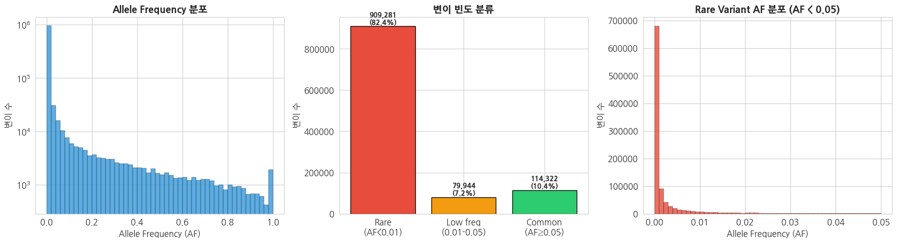

png

=== AF 기초 통계 ===
Mean AF: 0.0367
Median AF: 0.0004
Singleton (AF < 0.001): 706,103 (64.0%)

2.3 변이 위치 분포 (Chromosome 22)

python

# 변이 위치 밀도 분포
pos_array = np.array(positions)

fig, axes = plt.subplots(2, 1, figsize=(16, 8))

# 1. 변이 밀도 (1Mb 윈도우)
window_size = 1_000_000  # 1Mb
bins = np.arange(pos_array.min(), pos_array.max() + window_size, window_size)
counts_per_window, bin_edges = np.histogram(pos_array, bins=bins)
bin_centers = (bin_edges[:-1] + bin_edges[1:]) / 2 / 1_000_000  # Mb 단위

axes[0].fill_between(bin_centers, counts_per_window, alpha=0.6, color='#3498db')
axes[0].plot(bin_centers, counts_per_window, color='#2c3e50', linewidth=0.8)
axes[0].set_title('Chromosome 22 변이 밀도 (1Mb window)', fontsize=14, fontweight='bold')
axes[0].set_xlabel('Position (Mb)')
axes[0].set_ylabel('변이 수 / 1Mb')
axes[0].axhline(y=np.mean(counts_per_window), color='red', linestyle='--', alpha=0.7, label=f'Mean: {np.mean(counts_per_window):.0f}')
axes[0].legend()

# 2. 변이 간 거리 분포
if len(pos_array) > 1:
    distances = np.diff(np.sort(pos_array))
    axes[1].hist(distances, bins=100, color='#e74c3c', edgecolor='black', linewidth=0.2, alpha=0.8)
    axes[1].set_title('인접 변이 간 거리 분포', fontsize=14, fontweight='bold')
    axes[1].set_xlabel('Distance (bp)')
    axes[1].set_ylabel('빈도')
    axes[1].set_xlim(0, np.percentile(distances, 99))
    axes[1].axvline(x=np.median(distances), color='blue', linestyle='--', alpha=0.7,
                    label=f'Median: {np.median(distances):.0f} bp')
    axes[1].legend()

plt.tight_layout()
plt.show()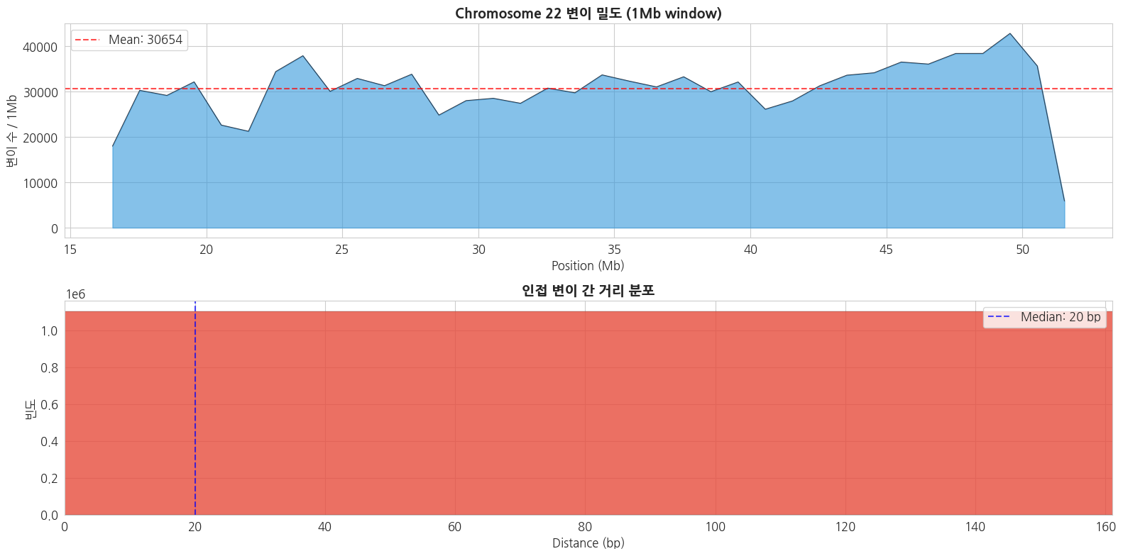

png

3. Mutation Profile 기반 변이 특성 요약

3.1 SNP 염기 치환 패턴 (Mutation Spectrum)

SNP는 6가지 기본 치환 유형으로 분류됩니다:

Transitions (Ts): A↔G, C↔T (퓨린↔퓨린 또는 피리미딘↔피리미딘)
Transversions (Tv): A↔C, A↔T, G↔C, G↔T

python

# SNP 치환 패턴 분석
vcf = VCF(VCF_PATH)

# 6가지 기본 치환 유형 (상보적 쌍 합산)
substitution_types = Counter()
# 12가지 세부 치환 유형
detailed_substitutions = Counter()
# Trinucleotide context (간략화: REF>ALT만)
ts_tv_count = {'Ts': 0, 'Tv': 0}

transitions = {('A', 'G'), ('G', 'A'), ('C', 'T'), ('T', 'C')}

for variant in vcf:
    if not variant.is_snp:
        continue
    
    ref = variant.REF
    for alt in variant.ALT:
        if len(ref) != 1 or len(alt) != 1:
            continue
        
        # 상세 치환
        detailed_substitutions[f'{ref}>{alt}'] += 1
        
        # 상보적 쌍 합산 (C:G>T:A 형태로 표준화)
        complement = {'A': 'T', 'T': 'A', 'C': 'G', 'G': 'C'}
        if ref in ('A', 'G'):
            ref_std = complement[ref]
            alt_std = complement[alt]
        else:
            ref_std = ref
            alt_std = alt
        substitution_types[f'{ref_std}>{alt_std}'] += 1
        
        # Ts/Tv
        if (ref, alt) in transitions:
            ts_tv_count['Ts'] += 1
        else:
            ts_tv_count['Tv'] += 1

vcf.close()

print('=== SNP 치환 유형 (6-class, 상보적 쌍 합산) ===')
for sub, count in sorted(substitution_types.items()):
    total_snps = sum(substitution_types.values())
    print(f'  {sub}: {count:,} ({count/total_snps*100:.1f}%)')

print(f'\n=== Ts/Tv ===')
print(f'Transitions: {ts_tv_count["Ts"]:,}')
print(f'Transversions: {ts_tv_count["Tv"]:,}')
print(f'Ts/Tv ratio: {ts_tv_count["Ts"]/ts_tv_count["Tv"]:.3f}')

=== SNP 치환 유형 (6-class, 상보적 쌍 합산) ===
  C>A: 95,912 (9.0%)
  C>G: 100,934 (9.5%)
  C>T: 510,426 (48.0%)
  T>A: 54,044 (5.1%)
  T>C: 239,112 (22.5%)
  T>G: 63,190 (5.9%)

=== Ts/Tv ===
Transitions: 749,538
Transversions: 314,080
Ts/Tv ratio: 2.386

python

# Mutation Spectrum 시각화
fig, axes = plt.subplots(1, 3, figsize=(20, 6))

# 1. 6-class 치환 유형 바 차트
sub_order = ['C>A', 'C>G', 'C>T', 'T>A', 'T>C', 'T>G']
sub_colors = ['#1ebff0', '#050708', '#e62725', '#cbcacb', '#a1cf64', '#edc8c5']
sub_vals = [substitution_types.get(s, 0) for s in sub_order]
total_snps = sum(sub_vals)

bars = axes[0].bar(sub_order, sub_vals, color=sub_colors, edgecolor='black', linewidth=0.5)
axes[0].set_title('SNP 치환 유형 (6-class)', fontsize=14, fontweight='bold')
axes[0].set_xlabel('Substitution Type')
axes[0].set_ylabel('변이 수')
for bar, val in zip(bars, sub_vals):
    axes[0].text(bar.get_x() + bar.get_width()/2, bar.get_height() + total_snps*0.005,
                f'{val/total_snps*100:.1f}%', ha='center', fontsize=10, fontweight='bold')

# 2. 12-class 세부 치환 바 차트
detail_order = ['A>C', 'A>G', 'A>T', 'C>A', 'C>G', 'C>T',
                'G>A', 'G>C', 'G>T', 'T>A', 'T>C', 'T>G']
detail_vals = [detailed_substitutions.get(s, 0) for s in detail_order]
detail_colors = ['#1ebff0', '#a1cf64', '#cbcacb', '#1ebff0', '#050708', '#e62725',
                 '#e62725', '#050708', '#1ebff0', '#cbcacb', '#a1cf64', '#edc8c5']

axes[1].bar(detail_order, detail_vals, color=detail_colors, edgecolor='black', linewidth=0.5)
axes[1].set_title('SNP 치환 유형 (12-class)', fontsize=14, fontweight='bold')
axes[1].set_xlabel('Substitution Type')
axes[1].set_ylabel('변이 수')
axes[1].tick_params(axis='x', rotation=45)

# 3. Ts/Tv 파이 차트
ts_tv_labels = ['Transition (Ts)', 'Transversion (Tv)']
ts_tv_vals = [ts_tv_count['Ts'], ts_tv_count['Tv']]
axes[2].pie(ts_tv_vals, labels=ts_tv_labels, autopct='%1.1f%%',
           colors=['#3498db', '#e74c3c'], startangle=90, textprops={'fontsize': 12})
axes[2].set_title(f'Transition / Transversion\n(Ts/Tv = {ts_tv_count["Ts"]/ts_tv_count["Tv"]:.3f})',
                  fontsize=14, fontweight='bold')

plt.tight_layout()
plt.show()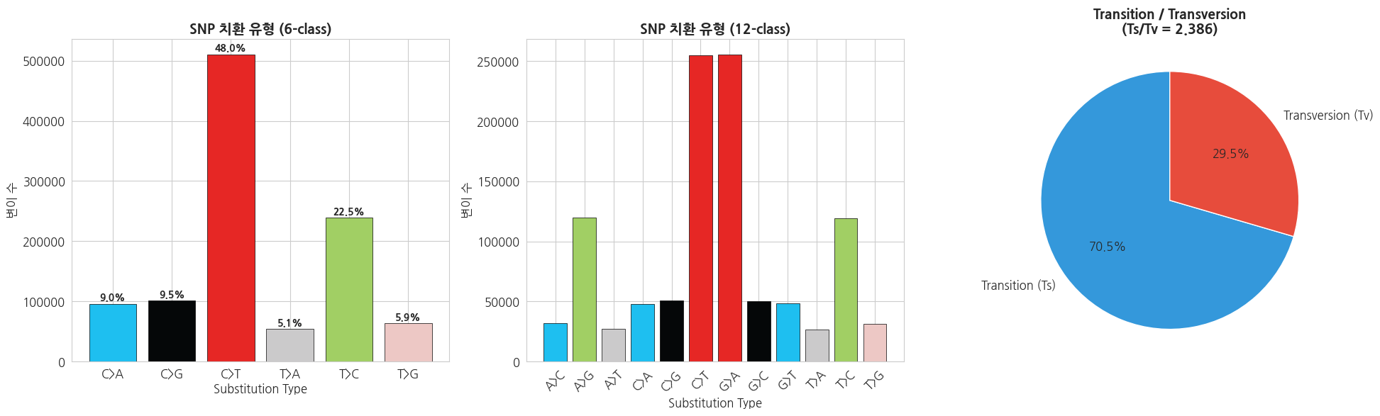

png

3.2 INDEL 크기 분포

python

# INDEL 크기 분석
vcf = VCF(VCF_PATH)

indel_sizes = []
for variant in vcf:
    if not variant.is_indel:
        continue
    for alt in variant.ALT:
        size = len(alt) - len(variant.REF)
        indel_sizes.append(size)

vcf.close()

indel_sizes = np.array(indel_sizes)

fig, axes = plt.subplots(1, 2, figsize=(16, 6))

# 1. INDEL 크기 전체 분포
axes[0].hist(indel_sizes, bins=range(min(indel_sizes)-1, max(min(max(indel_sizes), 50), 10)+2),
             color='#9b59b6', edgecolor='black', linewidth=0.3, alpha=0.8)
axes[0].set_title('INDEL 크기 분포', fontsize=14, fontweight='bold')
axes[0].set_xlabel('INDEL 크기 (bp, 양수=Insertion, 음수=Deletion)')
axes[0].set_ylabel('변이 수')
axes[0].axvline(x=0, color='red', linestyle='--', alpha=0.5)
axes[0].set_xlim(-30, 30)

# 2. INDEL 크기별 비율
size_categories = {
    '1 bp': np.sum(np.abs(indel_sizes) == 1),
    '2-5 bp': np.sum((np.abs(indel_sizes) >= 2) & (np.abs(indel_sizes) <= 5)),
    '6-10 bp': np.sum((np.abs(indel_sizes) >= 6) & (np.abs(indel_sizes) <= 10)),
    '11-20 bp': np.sum((np.abs(indel_sizes) >= 11) & (np.abs(indel_sizes) <= 20)),
    '>20 bp': np.sum(np.abs(indel_sizes) > 20)
}

cats = list(size_categories.keys())
cat_vals = list(size_categories.values())
axes[1].bar(cats, cat_vals, color=sns.color_palette('viridis', len(cats)), edgecolor='black', linewidth=0.5)
axes[1].set_title('INDEL 크기 범위별 분포', fontsize=14, fontweight='bold')
axes[1].set_xlabel('INDEL 크기 범위')
axes[1].set_ylabel('변이 수')
for i, (c, v) in enumerate(zip(cats, cat_vals)):
    axes[1].text(i, v + max(cat_vals)*0.01, f'{v:,}', ha='center', fontweight='bold', fontsize=10)

plt.tight_layout()
plt.show()

print(f'=== INDEL 크기 통계 ===')
print(f'전체 INDEL 수: {len(indel_sizes):,}')
print(f'Insertion: {np.sum(indel_sizes > 0):,}')
print(f'Deletion: {np.sum(indel_sizes < 0):,}')
print(f'평균 크기: {np.mean(np.abs(indel_sizes)):.1f} bp')
print(f'최대 Insertion: +{np.max(indel_sizes)} bp')
print(f'최대 Deletion: {np.min(indel_sizes)} bp')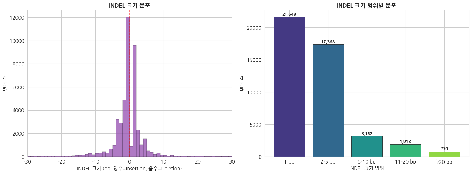

png

=== INDEL 크기 통계 ===
전체 INDEL 수: 45,750
Insertion: 17,035
Deletion: 27,831
평균 크기: 3.3 bp
최대 Insertion: +413 bp
최대 Deletion: -96 bp

3.3 Super Population별 변이 통계

python

# 1강에서 생성한 통합 데이터 로드
integrated = pd.read_csv(f'{DATA_DIR}/phenotype/integrated_sample_info.tsv', sep='\t')

# Super Population별 대표 샘플 1명씩 선택
representative_samples = {}
for sp in ['AFR', 'AMR', 'EAS', 'EUR', 'SAS']:
    sample = integrated[integrated['super_pop'] == sp]['sample'].values[0]
    representative_samples[sp] = sample

print('=== Super Population별 대표 샘플 ===')
for sp, sample in representative_samples.items():
    pop = integrated[integrated['sample'] == sample]['pop'].values[0]
    print(f'  {sp}: {sample} ({pop})')

=== Super Population별 대표 샘플 ===
  AFR: HG01879 (ACB)
  AMR: HG00551 (PUR)
  EAS: HG00403 (CHS)
  EUR: HG00096 (GBR)
  SAS: HG01583 (PJL)

python

# 각 대표 샘플별 개인 변이 수 계산
sample_variant_stats = {}

for sp, sample in representative_samples.items():
    # bcftools로 해당 샘플의 변이만 추출하여 카운트
    result = subprocess.run(
        ['bcftools', 'view', '-s', sample, '--min-ac', '1', '-H', VCF_PATH],
        capture_output=True, text=True
    )
    
    lines = [l for l in result.stdout.strip().split('\n') if l.strip()]
    total = len(lines)
    
    # SNP vs INDEL 분류
    snp = 0
    indel = 0
    for line in lines:
        fields = line.split('\t')
        if len(fields) < 5:
            continue
        ref = fields[3]
        alts = fields[4].split(',')
        if all(len(a) == 1 and len(ref) == 1 for a in alts):
            snp += 1
        else:
            indel += 1
    
    sample_variant_stats[sp] = {'total': total, 'SNP': snp, 'INDEL': indel}
    print(f'{sp} ({sample}): Total={total:,}, SNP={snp:,}, INDEL={indel:,}')

AFR (HG01879): Total=69,156, SNP=59,993, INDEL=9,163
AMR (HG00551): Total=55,633, SNP=47,802, INDEL=7,831
EAS (HG00403): Total=56,715, SNP=48,753, INDEL=7,962
EUR (HG00096): Total=54,175, SNP=46,477, INDEL=7,698
SAS (HG01583): Total=56,048, SNP=48,008, INDEL=8,040

python

# Super Population별 개인 변이 수 비교 시각화
sp_order = ['AFR', 'AMR', 'EAS', 'EUR', 'SAS']
sp_colors = {'AFR': '#e74c3c', 'AMR': '#f39c12', 'EAS': '#2ecc71', 'EUR': '#3498db', 'SAS': '#9b59b6'}

fig, axes = plt.subplots(1, 2, figsize=(16, 6))

# 1. 전체 변이 수 비교
totals = [sample_variant_stats[sp]['total'] for sp in sp_order]
colors = [sp_colors[sp] for sp in sp_order]
bars = axes[0].bar(sp_order, totals, color=colors, edgecolor='black', linewidth=0.5)
axes[0].set_title('Super Population별 개인 변이 수 (chr22)', fontsize=14, fontweight='bold')
axes[0].set_ylabel('변이 수')
for bar, val in zip(bars, totals):
    axes[0].text(bar.get_x() + bar.get_width()/2, bar.get_height() + max(totals)*0.01,
                f'{val:,}', ha='center', fontweight='bold')

# 2. SNP vs INDEL 비교 (stacked)
snps = [sample_variant_stats[sp]['SNP'] for sp in sp_order]
indels = [sample_variant_stats[sp]['INDEL'] for sp in sp_order]
x = np.arange(len(sp_order))
width = 0.6
axes[1].bar(x, snps, width, label='SNP', color='#3498db', edgecolor='black', linewidth=0.5)
axes[1].bar(x, indels, width, bottom=snps, label='INDEL', color='#e74c3c', edgecolor='black', linewidth=0.5)
axes[1].set_xticks(x)
axes[1].set_xticklabels(sp_order)
axes[1].set_title('Super Population별 SNP/INDEL 비교', fontsize=14, fontweight='bold')
axes[1].set_ylabel('변이 수')
axes[1].legend()

plt.tight_layout()
plt.show()

print('※ AFR(아프리카)이 가장 많은 변이를 보이는 것은 인류의 아프리카 기원과')
print('  아프리카 인구집단의 높은 유전적 다양성을 반영합니다.')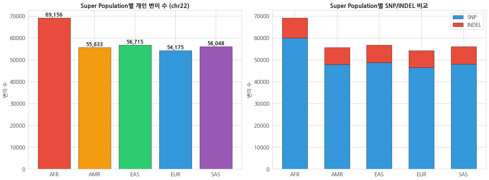

png

※ AFR(아프리카)이 가장 많은 변이를 보이는 것은 인류의 아프리카 기원과
  아프리카 인구집단의 높은 유전적 다양성을 반영합니다.

4. 필터링 조건별 변이 수 비교 분석

4.1 Allele Frequency 기반 필터링

python

# 다양한 MAF 기준으로 필터링 (bcftools 사용)
maf_thresholds = [0.001, 0.005, 0.01, 0.05, 0.1]
maf_results = {}

# 전체 변이 수
result = subprocess.run(
    ['bcftools', 'view', '-H', VCF_PATH],
    capture_output=True, text=True
)
total_count = len([l for l in result.stdout.strip().split('\n') if l.strip()])
maf_results['No filter'] = total_count

print(f'전체 변이 수 (필터 없음): {total_count:,}')
print()

for maf in maf_thresholds:
    # MAF >= threshold 인 변이 수
    result = subprocess.run(
        ['bcftools', 'view', '-q', f'{maf}:minor', '-H', VCF_PATH],
        capture_output=True, text=True
    )
    count = len([l for l in result.stdout.strip().split('\n') if l.strip()])
    maf_results[f'MAF≥{maf}'] = count
    print(f'MAF ≥ {maf}: {count:,} ({count/total_count*100:.1f}%)')

전체 변이 수 (필터 없음): 1,103,547

MAF ≥ 0.001: 395,235 (35.8%)
MAF ≥ 0.005: 241,737 (21.9%)
MAF ≥ 0.01: 191,544 (17.4%)
MAF ≥ 0.05: 110,835 (10.0%)
MAF ≥ 0.1: 84,321 (7.6%)

python

# MAF 필터링 결과 시각화
fig, axes = plt.subplots(1, 2, figsize=(16, 6))

# 1. 필터링 후 변이 수
labels = list(maf_results.keys())
values = list(maf_results.values())
colors_maf = plt.cm.RdYlGn(np.linspace(0.2, 0.8, len(labels)))

bars = axes[0].bar(labels, values, color=colors_maf, edgecolor='black', linewidth=0.5)
axes[0].set_title('MAF 필터링별 변이 수', fontsize=14, fontweight='bold')
axes[0].set_ylabel('변이 수')
axes[0].tick_params(axis='x', rotation=30)
for bar, val in zip(bars, values):
    axes[0].text(bar.get_x() + bar.get_width()/2, bar.get_height() + max(values)*0.01,
                f'{val:,}', ha='center', fontsize=9, fontweight='bold')

# 2. 필터링으로 제거되는 비율
retained_pct = [v/total_count*100 for v in values]
removed_pct = [100 - p for p in retained_pct]

axes[1].bar(labels, retained_pct, color='#2ecc71', edgecolor='black', linewidth=0.5, label='Retained')
axes[1].bar(labels, removed_pct, bottom=retained_pct, color='#e74c3c', edgecolor='black', linewidth=0.5, label='Removed')
axes[1].set_title('MAF 필터링별 Retained/Removed 비율', fontsize=14, fontweight='bold')
axes[1].set_ylabel('비율 (%)')
axes[1].tick_params(axis='x', rotation=30)
axes[1].legend()

plt.tight_layout()
plt.show()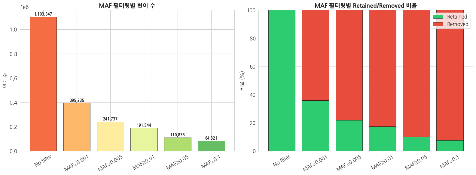

png

4.2 변이 타입별 필터링 (bcftools)

python

# SNP만 필터링
result = subprocess.run(
    ['bcftools', 'view', '-v', 'snps', '-H', VCF_PATH],
    capture_output=True, text=True
)
snp_only = len([l for l in result.stdout.strip().split('\n') if l.strip()])

# INDEL만 필터링
result = subprocess.run(
    ['bcftools', 'view', '-v', 'indels', '-H', VCF_PATH],
    capture_output=True, text=True
)
indel_only = len([l for l in result.stdout.strip().split('\n') if l.strip()])

# Biallelic만
result = subprocess.run(
    ['bcftools', 'view', '-m2', '-M2', '-H', VCF_PATH],
    capture_output=True, text=True
)
biallelic = len([l for l in result.stdout.strip().split('\n') if l.strip()])

# Multiallelic만
result = subprocess.run(
    ['bcftools', 'view', '-m3', '-H', VCF_PATH],
    capture_output=True, text=True
)
multiallelic = len([l for l in result.stdout.strip().split('\n') if l.strip()])

print('=== 변이 타입별 필터링 결과 ===')
filter_results = {
    '전체': total_count,
    'SNP only': snp_only,
    'INDEL only': indel_only,
    'Biallelic': biallelic,
    'Multiallelic': multiallelic
}

for name, count in filter_results.items():
    print(f'  {name:15s}: {count:>10,} ({count/total_count*100:5.1f}%)')

IOStream.flush timed out


=== 변이 타입별 필터링 결과 ===
  전체             :  1,103,547 (100.0%)
  SNP only       :  1,060,388 ( 96.1%)
  INDEL only     :     43,230 (  3.9%)
  Biallelic      :  1,097,199 ( 99.4%)
  Multiallelic   :      6,348 (  0.6%)

python

# 필터링 조합 비교 시각화
fig, ax = plt.subplots(figsize=(12, 6))

filter_names = list(filter_results.keys())
filter_counts = list(filter_results.values())
colors_filter = ['#34495e', '#3498db', '#e74c3c', '#2ecc71', '#f39c12']

bars = ax.barh(filter_names, filter_counts, color=colors_filter, edgecolor='black', linewidth=0.5)
ax.set_title('필터링 조건별 변이 수', fontsize=14, fontweight='bold')
ax.set_xlabel('변이 수')

for bar, val in zip(bars, filter_counts):
    ax.text(bar.get_width() + max(filter_counts)*0.01, bar.get_y() + bar.get_height()/2,
            f'{val:,} ({val/total_count*100:.1f}%)', va='center', fontweight='bold')

plt.tight_layout()
plt.show()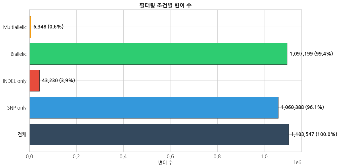

png

4.3 복합 필터링 전략 비교

python

# 다양한 필터링 조합 비교
filter_strategies = {
    '1. 전체 (No filter)': [],
    '2. SNP only': ['-v', 'snps'],
    '3. SNP + Biallelic': ['-v', 'snps', '-m2', '-M2'],
    '4. SNP + Biallelic + MAF≥0.01': ['-v', 'snps', '-m2', '-M2', '-q', '0.01:minor'],
    '5. SNP + Biallelic + MAF≥0.05': ['-v', 'snps', '-m2', '-M2', '-q', '0.05:minor'],
}

strategy_results = {}
for name, args in filter_strategies.items():
    cmd = ['bcftools', 'view', '-H'] + args + [VCF_PATH]
    result = subprocess.run(cmd, capture_output=True, text=True)
    count = len([l for l in result.stdout.strip().split('\n') if l.strip()])
    strategy_results[name] = count
    print(f'{name}: {count:,}')

1. 전체 (No filter): 1,103,547
2. SNP only: 1,060,388
3. SNP + Biallelic: 1,055,454
4. SNP + Biallelic + MAF≥0.01: 170,949
5. SNP + Biallelic + MAF≥0.05: 97,216

python

# 필터링 전략 비교 시각화 (파이프라인 형태)
fig, ax = plt.subplots(figsize=(14, 6))

names = list(strategy_results.keys())
counts = list(strategy_results.values())
colors_strat = plt.cm.Blues(np.linspace(0.3, 0.9, len(names)))

bars = ax.bar(range(len(names)), counts, color=colors_strat, edgecolor='black', linewidth=0.5)
ax.set_xticks(range(len(names)))
ax.set_xticklabels(names, rotation=15, ha='right', fontsize=10)
ax.set_title('필터링 전략별 변이 수 변화', fontsize=14, fontweight='bold')
ax.set_ylabel('변이 수')

# 감소율 표시
for i, (bar, count) in enumerate(zip(bars, counts)):
    ax.text(bar.get_x() + bar.get_width()/2, bar.get_height() + max(counts)*0.01,
            f'{count:,}', ha='center', fontweight='bold', fontsize=10)
    if i > 0:
        reduction = (1 - count/counts[i-1]) * 100
        ax.annotate(f'-{reduction:.1f}%',
                   xy=(i-0.5, (counts[i-1] + count)/2),
                   fontsize=9, color='red', fontweight='bold', ha='center')

plt.tight_layout()
plt.show()

print(f'\n전체 → 최종 필터링: {counts[0]:,} → {counts[-1]:,} ({counts[-1]/counts[0]*100:.1f}% retained)')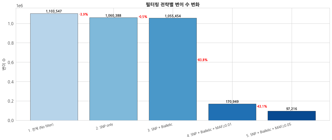

png

전체 → 최종 필터링: 1,103,547 → 97,216 (8.8% retained)

4.4 vcftools를 이용한 품질 통계

python

import os
import tempfile

# vcftools로 site-level 통계 계산
out_prefix = f'{DATA_DIR}/individual/chr22_stats'

# allele frequency 계산
subprocess.run(
    ['vcftools', '--gzvcf', VCF_PATH, '--freq', '--out', out_prefix],
    capture_output=True, text=True
)

# site depth (mean depth per site)
subprocess.run(
    ['vcftools', '--gzvcf', VCF_PATH, '--site-mean-depth', '--out', out_prefix],
    capture_output=True, text=True
)

# missingness per site
subprocess.run(
    ['vcftools', '--gzvcf', VCF_PATH, '--missing-site', '--out', out_prefix],
    capture_output=True, text=True
)

print('vcftools 통계 계산 완료!')
print(f'출력 파일 위치: {out_prefix}.*')

vcftools 통계 계산 완료!
출력 파일 위치: /tier4/DSC/jheepark/bbp-wgs-data/individual/chr22_stats.*

python

# vcftools 결과 시각화
fig, axes = plt.subplots(1, 3, figsize=(18, 5))

# 1. Allele Frequency 분포 (vcftools)
# .frq 파일은 multi-allelic 사이트에서 컬럼 수가 가변적이므로 라인 단위로 수동 파싱
freq_file = f'{out_prefix}.frq'
if os.path.exists(freq_file):
    minor_af = []
    with open(freq_file) as f:
        next(f)  # 헤더 스킵
        for line in f:
            fields = line.rstrip('\n').split('\t')
            if len(fields) < 5:
                continue
            # 5번째 컬럼부터가 allele:freq 반복 필드
            freqs = []
            for val in fields[4:]:
                if ':' in val:
                    try:
                        freqs.append(float(val.rsplit(':', 1)[1]))
                    except ValueError:
                        pass
            if freqs:
                minor_af.append(min(freqs))

    if minor_af:
        axes[0].hist(minor_af, bins=50, color='#3498db', edgecolor='black', linewidth=0.3)
        axes[0].set_title('Minor Allele Frequency 분포\n(vcftools)', fontsize=13, fontweight='bold')
        axes[0].set_xlabel('Minor Allele Frequency')
        axes[0].set_ylabel('변이 수')
        axes[0].set_yscale('log')

# 2. Site Mean Depth
# 1000 Genomes Phase 3 VCF에는 개별 샘플의 DP 정보가 없어 MEAN_DEPTH가 -nan으로 출력될 수 있음
depth_file = f'{out_prefix}.ldepth.mean'
if os.path.exists(depth_file):
    depth_df = pd.read_csv(depth_file, sep='\t', na_values=['-nan', 'nan', '-inf', 'inf'])
    if 'MEAN_DEPTH' in depth_df.columns:
        depth_vals = depth_df['MEAN_DEPTH'].dropna()
        if len(depth_vals) > 0:
            axes[1].hist(depth_vals, bins=50, color='#2ecc71', edgecolor='black', linewidth=0.3)
            axes[1].set_title('Site Mean Depth 분포\n(vcftools)', fontsize=13, fontweight='bold')
            axes[1].set_xlabel('Mean Depth')
            axes[1].set_ylabel('Site 수')
        else:
            axes[1].text(0.5, 0.5,
                         '1000 Genomes Phase 3 VCF에는\n개별 샘플의 DP 정보가 없어\nMEAN_DEPTH 산출 불가',
                         ha='center', va='center', transform=axes[1].transAxes, fontsize=12)
            axes[1].set_title('Site Mean Depth\n(데이터 없음)', fontsize=13, fontweight='bold')
            axes[1].set_xticks([])
            axes[1].set_yticks([])

# 3. Site Missingness
miss_file = f'{out_prefix}.lmiss'
if os.path.exists(miss_file):
    miss_df = pd.read_csv(miss_file, sep='\t')
    if 'F_MISS' in miss_df.columns:
        miss_vals = miss_df['F_MISS'].dropna()
        axes[2].hist(miss_vals, bins=50, color='#e74c3c', edgecolor='black', linewidth=0.3)
        axes[2].set_title('Site Missingness 분포\n(vcftools)', fontsize=13, fontweight='bold')
        axes[2].set_xlabel('Missingness Rate (F_MISS)')
        axes[2].set_ylabel('Site 수')
        axes[2].set_yscale('log')

plt.tight_layout()
plt.show()

# 요약 통계 출력
if minor_af:
    maf_arr = np.array(minor_af)
    print(f'=== vcftools 통계 요약 ===')
    print(f'Minor AF - 변이 수: {len(maf_arr):,}')
    print(f'Minor AF - Median: {np.median(maf_arr):.4f}, Mean: {maf_arr.mean():.4f}')
    print(f'Rare (MAF<0.01): {np.sum(maf_arr < 0.01):,} ({np.sum(maf_arr < 0.01)/len(maf_arr)*100:.1f}%)')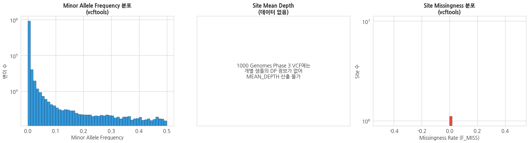

png

=== vcftools 통계 요약 ===
Minor AF - 변이 수: 1,103,547
Minor AF - Median: 0.0004, Mean: 0.0254
Rare (MAF<0.01): 912,003 (82.6%)

5. 요약 및 다음 강의 안내

이번 강의 요약

항목	내용
VCF 구조	8개 고정 컬럼 (CHROM, POS, ID, REF, ALT, QUAL, FILTER, INFO) + FORMAT/Genotype
변이 수	chr22 기준 약 100만개 이상 (2,504 샘플)
변이 타입	SNP가 다수, INDEL은 1bp 크기가 가장 흔함
Mutation Profile	C>T transition이 가장 빈번, Ts/Tv ~2.0
AF 분포	Rare variant (AF<0.01)가 대다수
인구집단 차이	AFR이 가장 높은 유전적 다양성 (변이 수 최다)

핵심 포인트

VCF 파일 구조 이해는 모든 유전체 분석의 기초입니다.
Ts/Tv 비율은 데이터 품질을 평가하는 중요한 지표입니다.
Rare variant가 대다수를 차지하며, 분석 목적에 맞는 필터링이 중요합니다.
bcftools, vcftools는 VCF 처리의 필수 도구입니다.
인구집단별 유전적 다양성 차이는 후속 분석에서 중요한 고려 사항입니다.

주요 bcftools 명령어 정리

bash

# 헤더 확인
bcftools view -h file.vcf.gz

# 기본 통계
bcftools stats file.vcf.gz

# SNP만 추출
bcftools view -v snps file.vcf.gz

# 특정 샘플 추출
bcftools view -s SAMPLE_ID file.vcf.gz

# MAF 필터링
bcftools view -q 0.05:minor file.vcf.gz

# Biallelic만 추출
bcftools view -m2 -M2 file.vcf.gz

다음 강의 예고

3강: 개인 기반 WGS 분석 및 실습

변이 주석(annotation) 결과 확인 및 해석
질환 관련 변이 선별 및 variant prioritization
암(Somatic)·희귀질환(Germline) 분석 결과 비교

2강: VCF 기초 통계 분석 ​

BBP WGS 분석 튜토리얼 ​

학습 목표 ​

사용 데이터 ​

산출물 (본 강의에서 생성) ​

사용 도구 ​

0. 환경 설정 ​

1. VCF 파일 구조 이해 ​

VCF (Variant Call Format) 파일이란? ​

VCF 파일 구성 ​

1.1 VCF 헤더 확인 ​

1.2 VCF 주요 8개 고정 컬럼 ​

1.3 bcftools stats로 기본 통계 확인 ​

2. SNP·INDEL 등 변이 타입 분포 시각화 ​

2.1 cyvcf2를 이용한 변이 타입 분류 ​

2.2 Allele Frequency (AF) 분포 ​

2.3 변이 위치 분포 (Chromosome 22) ​

3. Mutation Profile 기반 변이 특성 요약 ​

3.1 SNP 염기 치환 패턴 (Mutation Spectrum) ​

3.2 INDEL 크기 분포 ​

3.3 Super Population별 변이 통계 ​

4. 필터링 조건별 변이 수 비교 분석 ​

4.1 Allele Frequency 기반 필터링 ​

4.2 변이 타입별 필터링 (bcftools) ​

4.3 복합 필터링 전략 비교 ​

4.4 vcftools를 이용한 품질 통계 ​

5. 요약 및 다음 강의 안내 ​

이번 강의 요약 ​

핵심 포인트 ​

주요 bcftools 명령어 정리 ​

다음 강의 예고 ​

2강: VCF 기초 통계 분석

BBP WGS 분석 튜토리얼

학습 목표

사용 데이터

산출물 (본 강의에서 생성)

사용 도구

0. 환경 설정

1. VCF 파일 구조 이해

VCF (Variant Call Format) 파일이란?

VCF 파일 구성

1.1 VCF 헤더 확인

1.2 VCF 주요 8개 고정 컬럼

1.3 bcftools stats로 기본 통계 확인

2. SNP·INDEL 등 변이 타입 분포 시각화

2.1 cyvcf2를 이용한 변이 타입 분류

2.2 Allele Frequency (AF) 분포

2.3 변이 위치 분포 (Chromosome 22)

3. Mutation Profile 기반 변이 특성 요약

3.1 SNP 염기 치환 패턴 (Mutation Spectrum)

3.2 INDEL 크기 분포

3.3 Super Population별 변이 통계

4. 필터링 조건별 변이 수 비교 분석

4.1 Allele Frequency 기반 필터링

4.2 변이 타입별 필터링 (bcftools)

4.3 복합 필터링 전략 비교

4.4 vcftools를 이용한 품질 통계

5. 요약 및 다음 강의 안내

이번 강의 요약

핵심 포인트

주요 bcftools 명령어 정리

다음 강의 예고