3강: 개인 환자 유전체 기반 변이 해석

BBP WGS 분석 튜토리얼

학습 목표

변이 주석(Annotation) 결과 확인 및 해석 - ClinVar, 기능적 영향(Consequence) 기반 변이 주석
질환 관련 변이 선별 및 Variant Prioritization - 병원성 변이 필터링 및 우선순위화
암(Somatic)·희귀질환(Germline) 환자 해석 차이 비교 - 두 해석 전략의 실제 데이터 비교 분석

사용 데이터

데이터 루트: /tier4/DSC/jheepark/bbp-wgs-data/

Germline 트랙 (GRCh37)

데이터	경로	설명
1000 Genomes chr22 VCF	`individual/ALL.chr22.phase3_shapeit2_mvncall_integrated_v5b.20130502.genotypes.vcf.gz`	2,504 샘플 joint VCF. 여기서 개인 샘플(NA18939, JPT)을 추출
ClinVar VCF (GRCh37)	`annotation/clinvar.vcf.gz`	변이의 임상적 병원성 분류 정보
통합 샘플 정보	`phenotype/integrated_sample_info.tsv`	1강에서 생성한 Panel + Pedigree 병합 데이터

Somatic 트랙 (GRCh38)

데이터	경로	설명
HCC1395 Somatic VCF	`individual/somatic/HCC1395_somatic.chr22.vcf.gz`	SEQC2 consortium, 유방암 세포주 high-confidence somatic call set (chr22, 657개 변이)
ClinVar VCF (GRCh38)	`annotation/clinvar_GRCh38.vcf.gz`	GRCh38 기반 임상 병원성 정보
VEP cache (선택)	`annotation/vep/homo_sapiens/`	Docker 로컬 VEP 실행 시 필요. 최초 1회 ~15GB 다운로드

⚠️ Reference genome 차이: Germline 트랙은 GRCh37, Somatic 트랙은 GRCh38 입니다. 두 트랙을 각자의 reference 에 맞는 ClinVar 로 독립 annotation 한 뒤, 해석 결과 단계에서 비교합니다.

산출물 (본 강의에서 생성)

파일	경로	설명
환자 VCF (Germline)	`individual/patient_{SAMPLE}.vcf.gz`	단일 환자 변이만 추출
ClinVar 주석 VCF (Germline)	`individual/patient_{SAMPLE}.clinvar.vcf.gz`	ClinVar INFO 주입
VEP 입력 VCF	`individual/patient_{SAMPLE}.vep_input.vcf.gz`	VEP 실습용 소규모 변이 세트
Germline Prioritized TSV	`individual/patient_{SAMPLE}.prioritized.tsv`	최종 Germline 후보 변이
Germline P/LP TSV	`individual/patient_{SAMPLE}.germline_plp.tsv`	Germline Pathogenic/Likely pathogenic 변이
Somatic ClinVar VCF	`individual/HCC1395_somatic.clinvar.chr22.vcf.gz`	ClinVar GRCh38 주입
Somatic Prioritized TSV	`individual/HCC1395_somatic.prioritized.tsv`	HighConf + Coding impact 변이

사용 도구

bcftools, tabix (VCF 주석 주입 및 필터링)
Ensembl VEP (Docker / Singularity / Conda 설치 + Ensembl REST API)
Python: cyvcf2, pandas, requests, matplotlib, seaborn

0. 환경 설정

python

import os
import tempfile

# /tmp 공간 부족 시 FileNotFoundError 방지: 쓰기 가능한 임시 디렉토리 확보
def _ensure_tmpdir():
    for cand in [os.environ.get('TMPDIR'), '/tmp', '/var/tmp',
                 os.path.expanduser('~/.cache/tmp')]:
        if not cand:
            continue
        try:
            os.makedirs(cand, exist_ok=True)
            with tempfile.NamedTemporaryFile(dir=cand, delete=True):
                pass
            return cand
        except (OSError, PermissionError):
            continue
    raise RuntimeError('사용 가능한 임시 디렉토리를 찾지 못했습니다.')

_tmp = _ensure_tmpdir()
os.environ['TMPDIR'] = _tmp
tempfile.tempdir = _tmp
print(f'임시 디렉토리: {_tmp}')

import subprocess
import re
from collections import Counter, defaultdict

import pandas as pd
import numpy as np
import matplotlib
import matplotlib.pyplot as plt
import seaborn as sns
from cyvcf2 import VCF
from matplotlib import font_manager
import warnings
warnings.filterwarnings('ignore')

# 시각화 설정 (seaborn 스타일을 먼저 설정해야 한글 폰트가 덮어씌워지지 않음)
sns.set_style('whitegrid')
sns.set_palette('Set2')

# ============================================================
# 한글 폰트 설정 — NanumGothic 등록 + fallback chain + 캐시 갱신
# ============================================================
_KR_FONT = 'NanumGothic'
_KR_CANDIDATES = [
    '/usr/share/fonts/truetype/nanum/NanumGothic.ttf',
    '/usr/share/fonts/truetype/nanum/NanumBarunGothic.ttf',
    '/usr/share/fonts/truetype/nanum/NanumSquareR.ttf',
]
_registered = False
for _fp in _KR_CANDIDATES:
    if os.path.exists(_fp):
        try:
            font_manager.fontManager.addfont(_fp)
            _KR_FONT = font_manager.FontProperties(fname=_fp).get_name()
            _registered = True
            print(f'한글 폰트 등록: {_KR_FONT} ({_fp})')
            break
        except Exception as e:
            print(f'폰트 등록 실패: {_fp} - {e}')

if not _registered:
    print('⚠ 한글 폰트 파일을 찾지 못했습니다. 한글이 깨질 수 있습니다.')

# 전역 rcParams: sans-serif 체인의 맨 앞에 한글 폰트
plt.rcParams['font.family'] = 'sans-serif'
plt.rcParams['font.sans-serif'] = [_KR_FONT, 'DejaVu Sans', 'Liberation Sans', 'Arial']
plt.rcParams['axes.unicode_minus'] = False
plt.rcParams['figure.figsize'] = (12, 6)
plt.rcParams['font.size'] = 12
# 이미지 크기 초과(ValueError: Image size too large) 방지 - dpi 고정
plt.rcParams['figure.dpi'] = 100
plt.rcParams['savefig.dpi'] = 100
plt.rcParams['figure.autolayout'] = False

def safe_top(series_or_dict, n=30):
    """barh 시각화 전 상위 n개만 남겨 이미지 높이 폭주(>2^16 px) 방지."""
    if hasattr(series_or_dict, 'head'):
        return series_or_dict.head(n)
    if isinstance(series_or_dict, dict):
        items = list(series_or_dict.items())[:n]
        return dict(items)
    return series_or_dict

# 데이터 경로
DATA_DIR = '/tier4/DSC/jheepark/bbp-wgs-data'
INDIVIDUAL_DIR = f'{DATA_DIR}/individual'
SOMATIC_DIR   = f'{DATA_DIR}/individual/somatic'
ANNOTATION_DIR = f'{DATA_DIR}/annotation'
PHENOTYPE_DIR = f'{DATA_DIR}/phenotype'

# Germline (GRCh37) - 1000 Genomes chr22 + 환자 1명 추출용
VCF_PATH     = f'{INDIVIDUAL_DIR}/ALL.chr22.phase3_shapeit2_mvncall_integrated_v5b.20130502.genotypes.vcf.gz'
CLINVAR_PATH = f'{ANNOTATION_DIR}/clinvar.vcf.gz'           # GRCh37

# Somatic (GRCh38) - HCC1395 유방암 세포주 high-confidence somatic VCF
SOMATIC_VCF      = f'{SOMATIC_DIR}/HCC1395_somatic.chr22.vcf.gz'
CLINVAR_GRCH38   = f'{ANNOTATION_DIR}/clinvar_GRCh38.vcf.gz'

# 실습용 출력 경로
WORK_DIR = f'{INDIVIDUAL_DIR}'

print('환경 설정 완료!')
print(f'[Germline] 개인 VCF : {VCF_PATH}')
print(f'[Germline] ClinVar  : {CLINVAR_PATH}   (GRCh37)')
print(f'[Somatic]  HCC1395  : {SOMATIC_VCF}')
print(f'[Somatic]  ClinVar  : {CLINVAR_GRCH38}   (GRCh38)')

임시 디렉토리: /tmp
한글 폰트 등록: NanumGothic (/usr/share/fonts/truetype/nanum/NanumGothic.ttf)
환경 설정 완료!
[Germline] 개인 VCF : /tier4/DSC/jheepark/bbp-wgs-data/individual/ALL.chr22.phase3_shapeit2_mvncall_integrated_v5b.20130502.genotypes.vcf.gz
[Germline] ClinVar  : /tier4/DSC/jheepark/bbp-wgs-data/annotation/clinvar.vcf.gz   (GRCh37)
[Somatic]  HCC1395  : /tier4/DSC/jheepark/bbp-wgs-data/individual/somatic/HCC1395_somatic.chr22.vcf.gz
[Somatic]  ClinVar  : /tier4/DSC/jheepark/bbp-wgs-data/annotation/clinvar_GRCh38.vcf.gz   (GRCh38)

1. 변이 주석(Annotation) 개요

1.1 Annotation이란?

VCF 파일 자체는 변이의 위치와 염기 서열만 알려줄 뿐, 그 변이가 어떤 유전자에 속하는지, 단백질에 어떤 영향을 주는지, 질환과 관련이 있는지 등의 임상적 해석 정보는 포함하지 않습니다.

Annotation은 외부 데이터베이스의 정보를 변이에 부착하여 해석 가능한 형태로 만드는 과정입니다.

주석 유형	주요 도구/DB	제공 정보
기능적 영향	Ensembl VEP, SnpEff	missense, stop_gained, splice_site 등
임상적 병원성	ClinVar	Pathogenic / Benign / VUS 등
인구집단 빈도	gnomAD, 1000G	대규모 코호트에서 관찰된 AF
기능 예측	CADD, SIFT, PolyPhen	in-silico 병원성 예측 점수

1.2 ClinVar 데이터 구조

ClinVar VCF의 주요 INFO 필드를 먼저 살펴봅니다.

python

# ClinVar 헤더에서 주요 INFO 필드만 추출
result = subprocess.run(
    ['bcftools', 'view', '-h', CLINVAR_PATH],
    capture_output=True, text=True
)

header_lines = result.stdout.strip().split('\n')

key_fields = ['CLNSIG', 'CLNDN', 'CLNREVSTAT', 'CLNVC', 'GENEINFO', 'MC', 'ORIGIN', 'RS']

print('=== ClinVar 주요 INFO 필드 ===')
for line in header_lines:
    if line.startswith('##INFO'):
        for k in key_fields:
            if f'ID={k},' in line:
                # 필드 이름과 Description 추출
                desc = re.search(r'Description="([^"]+)"', line)
                print(f'\n[{k}]')
                print(f'  {desc.group(1) if desc else line}')
                break

=== ClinVar 주요 INFO 필드 ===

[CLNDN]
  ClinVar's preferred disease name for the concept specified by disease identifiers in CLNDISDB

[CLNREVSTAT]
  ClinVar review status of germline classification for the Variation ID

[CLNSIG]
  Aggregate germline classification for this single variant; multiple values are separated by a vertical bar

[CLNVC]
  Variant type

[GENEINFO]
  Gene(s) for the variant reported as gene symbol:gene id. The gene symbol and id are delimited by a colon (:) and each pair is delimited by a vertical bar (|)

[MC]
  comma separated list of molecular consequence in the form of Sequence Ontology ID|molecular_consequence

[ORIGIN]
  Allele origin. One or more of the following values may be added: 0 - unknown; 1 - germline; 2 - somatic; 4 - inherited; 8 - paternal; 16 - maternal; 32 - de-novo; 64 - biparental; 128 - uniparental; 256 - not-tested; 512 - tested-inconclusive; 1073741824 - other

[RS]
  dbSNP ID (i.e. rs number)

python

# ClinVar chr22 변이 수 확인
result = subprocess.run(
    ['bcftools', 'view', '-H', '-r', '22', CLINVAR_PATH],
    capture_output=True, text=True
)
n_clinvar_chr22 = len([l for l in result.stdout.strip().split('\n') if l.strip()])
print(f'ClinVar chr22 변이 수: {n_clinvar_chr22:,}')

# 앞 3개 샘플
lines = result.stdout.strip().split('\n')[:3]
print('\n=== ClinVar chr22 변이 예시 ===')
for line in lines:
    fields = line.split('\t')
    chrom, pos, vid, ref, alt = fields[0], fields[1], fields[2], fields[3], fields[4]
    info = fields[7]
    # 주요 필드 추출
    clnsig = re.search(r'CLNSIG=([^;]+)', info)
    gene = re.search(r'GENEINFO=([^;:]+)', info)
    clndn = re.search(r'CLNDN=([^;]+)', info)
    print(f'\n  {chrom}:{pos} {ref}>{alt}  (ClinVar ID: {vid})')
    print(f'    Gene     : {gene.group(1) if gene else "-"}')
    print(f'    CLNSIG   : {clnsig.group(1) if clnsig else "-"}')
    print(f'    CLNDN    : {(clndn.group(1) if clndn else "-")[:80]}')

ClinVar chr22 변이 수: 95,486

=== ClinVar chr22 변이 예시 ===

  22:16258221 C>T  (ClinVar ID: 3216855)
    Gene     : POTEH
    CLNSIG   : Uncertain_significance
    CLNDN    : not_specified

  22:16258239 C>T  (ClinVar ID: 3423174)
    Gene     : POTEH
    CLNSIG   : Uncertain_significance
    CLNDN    : not_specified

  22:16258254 C>T  (ClinVar ID: 4570584)
    Gene     : POTEH
    CLNSIG   : Likely_benign
    CLNDN    : not_specified

2. 개인 환자 샘플 선택 및 변이 주석

2.1 분석 대상 환자 선택

1강에서 생성한 통합 데이터에서 EAS 환자 1명을 선택합니다. 실제 임상에서는 환자의 WGS 결과 VCF가 분석 대상이 됩니다.

python

# 통합 데이터 로드
integrated = pd.read_csv(f'{PHENOTYPE_DIR}/integrated_sample_info.tsv', sep='\t')

# 분석 대상 환자 선택 (JPT 일본인)
target_sample = integrated[integrated['pop'] == 'JPT']['sample'].values[0]

print(f'=== 분석 대상 환자 ===')
print(f'  Sample ID      : {target_sample}')
print(f'  Population     : JPT (Japanese in Tokyo)')
print(f'  Super Population: EAS (East Asian)')

# 해당 샘플만 추출한 VCF 생성
patient_vcf = f'{WORK_DIR}/patient_{target_sample}.vcf.gz'

subprocess.run(
    ['bcftools', 'view', '-s', target_sample, '--min-ac', '1',
     '-Oz', '-o', patient_vcf, VCF_PATH],
    capture_output=True, text=True, check=True
)
subprocess.run(['tabix', '-p', 'vcf', '-f', patient_vcf],
               capture_output=True, text=True, check=True)

# 환자 변이 수 확인
result = subprocess.run(['bcftools', 'view', '-H', patient_vcf],
                        capture_output=True, text=True)
n_patient = len([l for l in result.stdout.strip().split('\n') if l.strip()])
print(f'\n환자 변이 수 (chr22): {n_patient:,}')
print(f'환자 VCF 저장: {patient_vcf}')

=== 분석 대상 환자 ===
  Sample ID      : NA18939
  Population     : JPT (Japanese in Tokyo)
  Super Population: EAS (East Asian)

환자 변이 수 (chr22): 56,754
환자 VCF 저장: /tier4/DSC/jheepark/bbp-wgs-data/individual/patient_NA18939.vcf.gz

2.2 ClinVar annotation 주입

bcftools annotate 를 이용해 환자 VCF에 ClinVar 정보를 추가합니다. 동일 position & REF/ALT 가 일치하는 변이에 대해 CLNSIG, CLNDN, GENEINFO 등이 부착됩니다.

python

# bcftools annotate 로 ClinVar INFO 주입
annotated_vcf = f'{WORK_DIR}/patient_{target_sample}.clinvar.vcf.gz'

# INFO 필드 선택적으로 가져오기
cmd = [
    'bcftools', 'annotate',
    '-a', CLINVAR_PATH,
    '-c', 'INFO/CLNSIG,INFO/CLNDN,INFO/CLNREVSTAT,INFO/GENEINFO,INFO/MC,INFO/ORIGIN',
    '-Oz', '-o', annotated_vcf,
    patient_vcf
]
result = subprocess.run(cmd, capture_output=True, text=True)
subprocess.run(['tabix', '-p', 'vcf', '-f', annotated_vcf],
               capture_output=True, text=True)

print('ClinVar annotation 완료')
print(f'출력 파일: {annotated_vcf}')

# 주입된 변이 수 확인 (CLNSIG가 있는 것만)
result = subprocess.run(
    ['bcftools', 'view', '-i', 'INFO/CLNSIG!="."', '-H', annotated_vcf],
    capture_output=True, text=True
)
n_annotated = len([l for l in result.stdout.strip().split('\n') if l.strip()])
print(f'\n환자 변이 {n_patient:,}개 중 ClinVar 주석이 부착된 변이: {n_annotated:,} ({n_annotated/n_patient*100:.2f}%)')

ClinVar annotation 완료
출력 파일: /tier4/DSC/jheepark/bbp-wgs-data/individual/patient_NA18939.clinvar.vcf.gz

환자 변이 56,754개 중 ClinVar 주석이 부착된 변이: 1,008 (1.78%)

2.3 Ensembl VEP 설치 및 간단한 Annotation 실습

Ensembl VEP (Variant Effect Predictor) 는 변이의 기능적 결과(consequence) 를 예측하는 표준 도구입니다. ClinVar 가 "이 변이가 어떤 질환인가"에 답한다면, VEP 는 "이 변이가 어느 유전자의 어떤 위치에 있으며 단백질을 어떻게 바꾸는가" 에 답합니다.

설치 방법 (3가지 중 택일)

방법	장점	단점
Docker	환경 충돌 없음, 빠른 설치	Docker 권한 필요
Singularity	HPC 환경 권장, sudo 불필요	이미지 빌드 시간
Conda/Source	플러그인 튜닝 용이	Perl 의존성 많음

① Docker 설치 (권장)

bash

# VEP Docker 이미지 pull
docker pull ensemblorg/ensembl-vep:release_110.1

# VEP cache/data 보관 디렉토리
VEP_DATA=/tier4/DSC/jheepark/bbp-wgs-data/annotation/vep
mkdir -p ${VEP_DATA}
chmod 777 ${VEP_DATA}    # 컨테이너 내부 사용자가 쓰기 가능하도록

# GRCh37 cache + fasta 다운로드 (최초 1회, ~15GB)
docker run -t -i --rm \
    -v ${VEP_DATA}:/opt/vep/.vep \
    ensemblorg/ensembl-vep:release_110.1 \
    INSTALL.pl -a cf -s homo_sapiens -y GRCh37 --NO_UPDATE

② Singularity 설치 (HPC 환경)

bash

singularity pull vep.sif docker://ensemblorg/ensembl-vep:release_110.1
singularity exec -B ${VEP_DATA}:/opt/vep/.vep vep.sif \
    INSTALL.pl -a cf -s homo_sapiens -y GRCh37 --NO_UPDATE

③ Conda 설치

bash

conda create -n vep -c bioconda ensembl-vep=110 -y
conda activate vep
vep_install -a cf -s homo_sapiens -y GRCh37 -c ${VEP_DATA} --NO_UPDATE

설치 확인

bash

docker run --rm ensemblorg/ensembl-vep:release_110.1 vep --help | head -5

VEP 주요 Consequence 범주

Impact	Consequence	설명
HIGH	stop_gained, frameshift_variant, splice_acceptor_variant, splice_donor_variant	단백질 기능 크게 망가짐
MODERATE	missense_variant, inframe_insertion, inframe_deletion, protein_altering_variant	아미노산 변화
LOW	synonymous_variant, splice_region_variant	서열 보존되나 주변 영향
MODIFIER	intron_variant, intergenic_variant, 5/3_prime_UTR_variant	비-코딩 영역

간단한 VEP Annotation 실습

VEP cache 다운로드(~15GB)에는 시간이 많이 소요되므로, 이 튜토리얼에서는 두 가지 경량 실습을 수행합니다.

입력 VCF 준비 — 환자 VCF에서 ClinVar Pathogenic 변이 5개만 추출
Docker VEP 명령어 확인 — 로컬에 VEP가 설치되어 있으면 바로 실행
Ensembl REST API 실습 — 네트워크만 되면 즉시 annotation (cache 불필요)

python

# VEP 입력용 소규모 VCF 생성
# 환자는 common 집단이라 Pathogenic 변이가 없을 수 있으므로
# 의미있는 ClinVar 주석(Pathogenic / drug_response / risk_factor / Conflicting 등)
# 이 부착된 변이 중 앞 5개를 선택
vep_input_vcf = f'{WORK_DIR}/patient_{target_sample}.vep_input.vcf.gz'

cmd = ['bcftools', 'view', '-i', 'INFO/CLNSIG!="."', annotated_vcf]
result = subprocess.run(cmd, capture_output=True, text=True)
lines = result.stdout.split('\n')

header = [l for l in lines if l.startswith('#')]
body_all = [l for l in lines if l and not l.startswith('#')]

# 우선순위: Pathogenic > drug_response > risk_factor > Conflicting > Uncertain > 기타
def priority(line):
    info = line.split('\t')[7]
    if 'CLNSIG=Pathogenic' in info and 'Benign' not in info: return 1
    if 'Likely_pathogenic' in info and 'Benign' not in info: return 2
    if 'drug_response' in info:      return 3
    if 'risk_factor'   in info:      return 4
    if 'Conflicting'   in info:      return 5
    if 'Uncertain'     in info:      return 6
    return 9

body_sorted = sorted(body_all, key=priority)
body = body_sorted[:5]

# 쓰기 + bgzip + tabix
plain_path = f'{WORK_DIR}/patient_{target_sample}.vep_input.vcf'
with open(plain_path, 'w') as f:
    f.write('\n'.join(header + body) + '\n')

subprocess.run(['bgzip', '-f', plain_path], check=True)
subprocess.run(['tabix', '-p', 'vcf', '-f', vep_input_vcf], check=True)

print(f'VEP 입력 VCF 생성: {vep_input_vcf}')
print(f'변이 수: {len(body)}')
print('\n=== 입력 변이 미리보기 ===')
for line in body:
    fields = line.split('\t')
    gene   = re.search(r'GENEINFO=([^;:]+)', fields[7])
    clnsig = re.search(r'CLNSIG=([^;]+)', fields[7])
    print(f'  {fields[0]}:{fields[1]} {fields[3]}>{fields[4]}  '
          f'Gene={gene.group(1) if gene else "-"}  '
          f'CLNSIG={clnsig.group(1) if clnsig else "-"}')

VEP 입력 VCF 생성: /tier4/DSC/jheepark/bbp-wgs-data/individual/patient_NA18939.vep_input.vcf.gz
변이 수: 5

=== 입력 변이 미리보기 ===
  22:19956781 G>A  Gene=ARVCF  CLNSIG=drug_response
  22:19957023 C>T  Gene=ARVCF  CLNSIG=drug_response
  22:42522312 T>C  Gene=CYP2D6  CLNSIG=drug_response
  22:42522392 G>A  Gene=CYP2D6  CLNSIG=drug_response
  22:42523209 T>C  Gene=CYP2D6  CLNSIG=drug_response

방법 A — Docker 로 VEP 로컬 실행 (cache 설치된 경우)

bash

# 실행 전 조건
# - Docker 이미지: ensemblorg/ensembl-vep:release_110.1
# - Cache: ${VEP_DATA}/homo_sapiens/110_GRCh37/

PATIENT_DIR=/tier4/DSC/jheepark/bbp-wgs-data/individual
VEP_DATA=/tier4/DSC/jheepark/bbp-wgs-data/annotation/vep

docker run --rm \
    -v ${PATIENT_DIR}:/data \
    -v ${VEP_DATA}:/opt/vep/.vep \
    ensemblorg/ensembl-vep:release_110.1 \
    vep \
      --input_file  /data/patient_NA18939.vep_input.vcf.gz \
      --output_file /data/patient_NA18939.vep.tsv \
      --cache --offline --assembly GRCh37 \
      --symbol --canonical --biotype \
      --sift b --polyphen b \
      --tab --force_overwrite

아래 셀은 Docker + cache 가 준비된 환경에서만 정상 작동합니다. 가용하지 않으면 건너뛰고 방법 B (REST API) 로 진행하세요.

python

# Docker + VEP cache 환경 여부 확인 후 실행
VEP_DATA = f'{ANNOTATION_DIR}/vep'
vep_cache_exists = os.path.isdir(f'{VEP_DATA}/homo_sapiens')
docker_exists = subprocess.run(['which', 'docker'], capture_output=True).returncode == 0

vep_tsv = f'{WORK_DIR}/patient_{target_sample}.vep.tsv'

if docker_exists and vep_cache_exists:
    cmd = [
        'docker', 'run', '--rm',
        '-v', f'{WORK_DIR}:/data',
        '-v', f'{VEP_DATA}:/opt/vep/.vep',
        'ensemblorg/ensembl-vep:release_110.1',
        'vep',
        '--input_file',  f'/data/patient_{target_sample}.vep_input.vcf.gz',
        '--output_file', f'/data/patient_{target_sample}.vep.tsv',
        '--cache', '--offline', '--assembly', 'GRCh37',
        '--symbol', '--canonical', '--biotype',
        '--sift', 'b', '--polyphen', 'b',
        '--tab', '--force_overwrite'
    ]
    print('[VEP Docker 실행 중...]')
    r = subprocess.run(cmd, capture_output=True, text=True)
    print(f'rc={r.returncode}')
    if r.returncode == 0:
        # TSV 파싱
        vep_df = pd.read_csv(vep_tsv, sep='\t', comment='#', header=None)
        print(f'VEP annotation 수: {len(vep_df)} 행')
        print(vep_df.head())
    else:
        print(r.stderr[:500])
else:
    missing = []
    if not docker_exists: missing.append('docker CLI')
    if not vep_cache_exists: missing.append(f'VEP cache ({VEP_DATA}/homo_sapiens)')
    print(f'[SKIP] 실행 조건 미충족: {", ".join(missing)}')
    print('→ 아래 방법 B (REST API) 로 진행하세요.')

[SKIP] 실행 조건 미충족: VEP cache (/tier4/DSC/jheepark/bbp-wgs-data/annotation/vep/homo_sapiens)
→ 아래 방법 B (REST API) 로 진행하세요.

방법 B — Ensembl REST API 로 즉시 Annotation (cache 불필요)

Ensembl 은 VEP 엔진을 REST API 로 공개합니다. 네트워크만 되면 누구나 사용 가능하며, 입력 변이를 chr pos . ref alt . . . 형식 (VCF-style) 으로 보내면 VEP 와 동일한 consequence 를 반환합니다.

엔드포인트 (GRCh37): https://grch37.rest.ensembl.org/vep/human/region
엔드포인트 (GRCh38): https://rest.ensembl.org/vep/human/region
요율 제한: 15 req/sec, per request ≤ 200 variants

python

import json
import requests

# REST API 입력 준비 - VCF-style 문자열 리스트
variants_for_rest = []
for line in body:
    fields = line.split('\t')
    chrom, pos, vid, ref, alt = fields[0], fields[1], fields[2], fields[3], fields[4]
    # REST API 형식: "chr pos id ref alt . . ."
    variants_for_rest.append(f'{chrom} {pos} {vid if vid != "." else "variant"} {ref} {alt} . . .')

print(f'REST API 로 보낼 변이 수: {len(variants_for_rest)}')
for v in variants_for_rest:
    print(f'  {v}')

# Ensembl REST API 호출 (GRCh37)
url = 'https://grch37.rest.ensembl.org/vep/human/region'
headers = {'Content-Type': 'application/json', 'Accept': 'application/json'}
payload = {'variants': variants_for_rest}

try:
    r = requests.post(url, headers=headers, data=json.dumps(payload), timeout=30)
    r.raise_for_status()
    vep_results = r.json()
    print(f'\n✓ VEP REST API 응답 수신 - {len(vep_results)} 변이')
except Exception as e:
    print(f'\n✗ REST API 호출 실패: {e}')
    print('  네트워크 상태를 확인하거나 방법 A(로컬 VEP) 를 사용하세요.')
    vep_results = []

REST API 로 보낼 변이 수: 5
  22 19956781 variant G A . . .
  22 19957023 variant C T . . .
  22 42522312 variant T C . . .
  22 42522392 variant G A . . .
  22 42523209 variant T C . . .

✓ VEP REST API 응답 수신 - 5 변이

python

# VEP REST API 응답 파싱 - 변이별 most_severe_consequence + 대표 transcript 정보
vep_rows = []
for res in vep_results:
    # 변이 기본 정보
    seq_region = res.get('seq_region_name')
    start      = res.get('start')
    input_str  = res.get('input', '')
    most_severe = res.get('most_severe_consequence')
    # 가장 영향이 큰 transcript consequence 선택 (canonical 우선)
    tc_list = res.get('transcript_consequences', [])
    canonical = [t for t in tc_list if t.get('canonical') == 1]
    best = canonical[0] if canonical else (tc_list[0] if tc_list else {})

    vep_rows.append({
        'input': input_str,
        'region': f'{seq_region}:{start}',
        'most_severe_consequence': most_severe,
        'gene_symbol': best.get('gene_symbol'),
        'transcript_id': best.get('transcript_id'),
        'impact': best.get('impact'),
        'biotype': best.get('biotype'),
        'canonical': best.get('canonical', 0),
        'hgvsc': best.get('hgvsc'),
        'hgvsp': best.get('hgvsp'),
        'sift_prediction':     best.get('sift_prediction'),
        'polyphen_prediction': best.get('polyphen_prediction'),
    })

vep_rest_df = pd.DataFrame(vep_rows)
print(f'VEP REST 결과 ({len(vep_rest_df)} 변이)\n')
cols_show = ['region', 'most_severe_consequence', 'impact', 'gene_symbol',
             'hgvsp', 'sift_prediction', 'polyphen_prediction']
print(vep_rest_df[cols_show].to_string(index=False))

VEP REST 결과 (5 변이)

     region most_severe_consequence   impact gene_symbol hgvsp sift_prediction polyphen_prediction
22:19956781     3_prime_UTR_variant MODIFIER        COMT  None            None                None
22:19957023     3_prime_UTR_variant MODIFIER        COMT  None            None                None
22:42522312          intron_variant MODIFIER      CYP2D6  None            None                None
22:42522392          intron_variant MODIFIER      CYP2D6  None            None                None
22:42523209          intron_variant MODIFIER      CYP2D6  None            None                None

VEP 결과와 ClinVar 결과 비교

VEP 의 Consequence/Impact 는 변이의 기능적 영향을, ClinVar 의 CLNSIG 는 임상적 병원성을 나타냅니다. 두 정보를 결합해 보면 해석의 신뢰도가 크게 올라갑니다.

python

# VEP REST 결과와 ClinVar 주석을 변이 단위로 결합
if len(vep_rest_df) == 0:
    print('VEP REST 결과가 없어 비교를 건너뜁니다.')
else:
    # body 에 들어있는 ClinVar 주석을 파싱 - 같은 순서로 매칭
    clinvar_rows = []
    for line in body:
        fields = line.split('\t')
        info = fields[7]
        gene   = re.search(r'GENEINFO=([^;:]+)', info)
        clnsig = re.search(r'CLNSIG=([^;]+)', info)
        clndn  = re.search(r'CLNDN=([^;]+)', info)
        clinvar_rows.append({
            'region': f'{fields[0]}:{fields[1]}',
            'clinvar_gene': gene.group(1) if gene else None,
            'clinvar_CLNSIG': clnsig.group(1) if clnsig else None,
            'clinvar_disease': (clndn.group(1) if clndn else '').replace('_', ' ')[:60],
        })
    clinvar_df = pd.DataFrame(clinvar_rows)

    # region 기반 merge
    merged = vep_rest_df.merge(clinvar_df, on='region', how='left')

    print('=== VEP + ClinVar 통합 해석 ===\n')
    for _, row in merged.iterrows():
        print(f'[{row["region"]}]')
        print(f'  VEP consequence : {row["most_severe_consequence"]} ({row["impact"]})')
        print(f'  VEP gene / HGVS : {row["gene_symbol"]}  {row["hgvsp"] or row["hgvsc"] or ""}')
        print(f'  VEP in-silico   : SIFT={row["sift_prediction"]}, PolyPhen={row["polyphen_prediction"]}')
        print(f'  ClinVar CLNSIG  : {row["clinvar_CLNSIG"]}')
        print(f'  ClinVar disease : {row["clinvar_disease"]}')
        print()

=== VEP + ClinVar 통합 해석 ===

[22:19956781]
  VEP consequence : 3_prime_UTR_variant (MODIFIER)
  VEP gene / HGVS : COMT  
  VEP in-silico   : SIFT=None, PolyPhen=None
  ClinVar CLNSIG  : drug_response
  ClinVar disease : Tramadol response

[22:19957023]
  VEP consequence : 3_prime_UTR_variant (MODIFIER)
  VEP gene / HGVS : COMT  
  VEP in-silico   : SIFT=None, PolyPhen=None
  ClinVar CLNSIG  : drug_response
  ClinVar disease : Tramadol response

[22:42522312]
  VEP consequence : intron_variant (MODIFIER)
  VEP gene / HGVS : CYP2D6  
  VEP in-silico   : SIFT=None, PolyPhen=None
  ClinVar CLNSIG  : drug_response
  ClinVar disease : Tramadol response

[22:42522392]
  VEP consequence : intron_variant (MODIFIER)
  VEP gene / HGVS : CYP2D6  
  VEP in-silico   : SIFT=None, PolyPhen=None
  ClinVar CLNSIG  : drug_response
  ClinVar disease : Tramadol response

[22:42523209]
  VEP consequence : intron_variant (MODIFIER)
  VEP gene / HGVS : CYP2D6  
  VEP in-silico   : SIFT=None, PolyPhen=None
  ClinVar CLNSIG  : drug_response
  ClinVar disease : Tramadol response

3. 주석 결과 파싱 및 해석

cyvcf2 로 annotated VCF 를 순회하며 CLNSIG / GENEINFO / MC 정보를 추출합니다.

python

# 주석된 환자 변이 파싱
records = []

vcf = VCF(annotated_vcf)
for v in vcf:
    clnsig = v.INFO.get('CLNSIG')
    if clnsig is None:
        continue
    gene = v.INFO.get('GENEINFO')
    gene_sym = gene.split(':')[0] if gene else None
    clndn = v.INFO.get('CLNDN')
    revstat = v.INFO.get('CLNREVSTAT')
    mc = v.INFO.get('MC')
    # MC 의 첫 consequence 만 추출 (e.g. "SO:0001583|missense_variant")
    consequence = None
    if mc:
        for token in mc.split(','):
            if '|' in token:
                consequence = token.split('|')[1]
                break
    origin = v.INFO.get('ORIGIN')

    # 환자의 genotype
    gt = v.genotypes[0] if len(v.genotypes) else [0, 0, False]
    alt_count = sum(1 for a in gt[:2] if a == 1)
    zygosity = 'hom_alt' if alt_count == 2 else ('het' if alt_count == 1 else 'hom_ref')

    records.append({
        'CHROM': v.CHROM,
        'POS': v.POS,
        'REF': v.REF,
        'ALT': v.ALT[0] if v.ALT else '.',
        'rsID': v.ID,
        'GENE': gene_sym,
        'CLNSIG': clnsig,
        'CLNDN': clndn,
        'CLNREVSTAT': revstat,
        'CONSEQUENCE': consequence,
        'ORIGIN': origin,
        'ZYGOSITY': zygosity,
    })
vcf.close()

ann_df = pd.DataFrame(records)
print(f'ClinVar 주석이 부착된 환자 변이: {len(ann_df):,}개')
ann_df.head(10)

ClinVar 주석이 부착된 환자 변이: 1,008개

	CHROM	POS	REF	ALT	rsID	GENE	CLNSIG	CLNDN	CLNREVSTAT	CONSEQUENCE	ORIGIN	ZYGOSITY
0	22	17565888	C	A	None	IL17RA	Benign	not_provided\|not_specified	criteria_provided,_multiple_submitters,_no_con...	None	1	het
1	22	17565932	T	C	None	IL17RA	Benign	not_specified\|not_provided	criteria_provided,_multiple_submitters,_no_con...	5_prime_UTR_variant	1	hom_alt
2	22	17565974	G	C	None	IL17RA	Benign	Immunodeficiency_51\|not_specified\|not_provided	criteria_provided,_multiple_submitters,_no_con...	5_prime_UTR_variant	1	hom_alt
3	22	17566206	G	T	None	IL17RA	Benign	not_specified	criteria_provided,_single_submitter	intron_variant	1	hom_alt
4	22	17566229	T	A	None	IL17RA	Benign	not_specified	criteria_provided,_single_submitter	intron_variant	1	hom_alt
5	22	17582877	G	T	None	IL17RA	Benign/Likely_benign	not_specified\|not_provided\|Immunodeficiency_51	criteria_provided,_multiple_submitters,_no_con...	intron_variant	1	het
6	22	17586471	C	T	None	IL17RA	Benign	not_provided\|Immunodeficiency_51\|not_specified	criteria_provided,_multiple_submitters,_no_con...	intron_variant	1	het
7	22	17586583	C	G	None	IL17RA	Benign	not_specified	criteria_provided,_single_submitter	intron_variant	1	het
8	22	17586631	G	A	None	IL17RA	Benign	not_specified	criteria_provided,_single_submitter	intron_variant	1	het
9	22	17589516	C	T	None	IL17RA	Conflicting_classifications_of_pathogenicity	Immunodeficiency_51	criteria_provided,_conflicting_classifications	synonymous_variant	1	het

3.1 CLNSIG (병원성 분류) 분포

python

# CLNSIG 정규화 - 복합 값 처리
def normalize_clnsig(sig):
    if not sig:
        return 'Unknown'
    s = sig.replace('_', ' ')
    # 주요 카테고리 매핑
    if 'Pathogenic' in s and 'Conflicting' not in s:
        if 'Likely' in s:
            return 'Likely pathogenic'
        return 'Pathogenic'
    if 'Benign' in s and 'Conflicting' not in s:
        if 'Likely' in s:
            return 'Likely benign'
        return 'Benign'
    if 'Uncertain' in s:
        return 'VUS (Uncertain significance)'
    if 'Conflicting' in s:
        return 'Conflicting interpretations'
    if 'risk factor' in s.lower():
        return 'Risk factor'
    if 'drug response' in s.lower():
        return 'Drug response'
    return 'Other'

ann_df['CLNSIG_group'] = ann_df['CLNSIG'].apply(normalize_clnsig)

sig_counts = ann_df['CLNSIG_group'].value_counts()
print('=== 환자 변이의 CLNSIG 분포 ===')
for k, v in sig_counts.items():
    print(f'  {k:35s}: {v:>6,}')

=== 환자 변이의 CLNSIG 분포 ===
  Benign                             :    946
  Drug response                      :     22
  Other                              :     20
  Likely benign                      :      9
  VUS (Uncertain significance)       :      5
  Conflicting interpretations        :      4
  Risk factor                        :      2

python

# CLNSIG 분포 시각화
fig, axes = plt.subplots(1, 2, figsize=(16, 6), dpi=100)

# 색상 (병원성 → 경증)
sig_order = ['Pathogenic', 'Likely pathogenic', 'Conflicting interpretations',
             'VUS (Uncertain significance)', 'Risk factor', 'Drug response',
             'Likely benign', 'Benign', 'Other']
sig_colors = {
    'Pathogenic': '#c0392b',
    'Likely pathogenic': '#e74c3c',
    'Conflicting interpretations': '#e67e22',
    'VUS (Uncertain significance)': '#f1c40f',
    'Risk factor': '#9b59b6',
    'Drug response': '#8e44ad',
    'Likely benign': '#27ae60',
    'Benign': '#16a085',
    'Other': '#95a5a6',
}
present = [s for s in sig_order if s in sig_counts.index]
vals = [sig_counts[s] for s in present]
colors = [sig_colors[s] for s in present]

bars = axes[0].barh(present, vals, color=colors, edgecolor='black', linewidth=0.5)
axes[0].set_title('환자 변이의 ClinVar CLNSIG 분포', fontsize=14, fontweight='bold')
axes[0].set_xlabel('변이 수')
axes[0].invert_yaxis()
for bar, val in zip(bars, vals):
    axes[0].text(bar.get_width() + max(vals)*0.01, bar.get_y() + bar.get_height()/2,
                 f'{val:,}', va='center', fontweight='bold', fontsize=10)

# Consequence 분포 (상위 10개)
cons_counts = ann_df['CONSEQUENCE'].dropna().value_counts().head(10)
axes[1].barh(cons_counts.index[::-1], cons_counts.values[::-1],
             color='#3498db', edgecolor='black', linewidth=0.5)
axes[1].set_title('Molecular Consequence (상위 10개)', fontsize=14, fontweight='bold')
axes[1].set_xlabel('변이 수')

fig.tight_layout()
plt.show()
plt.close(fig)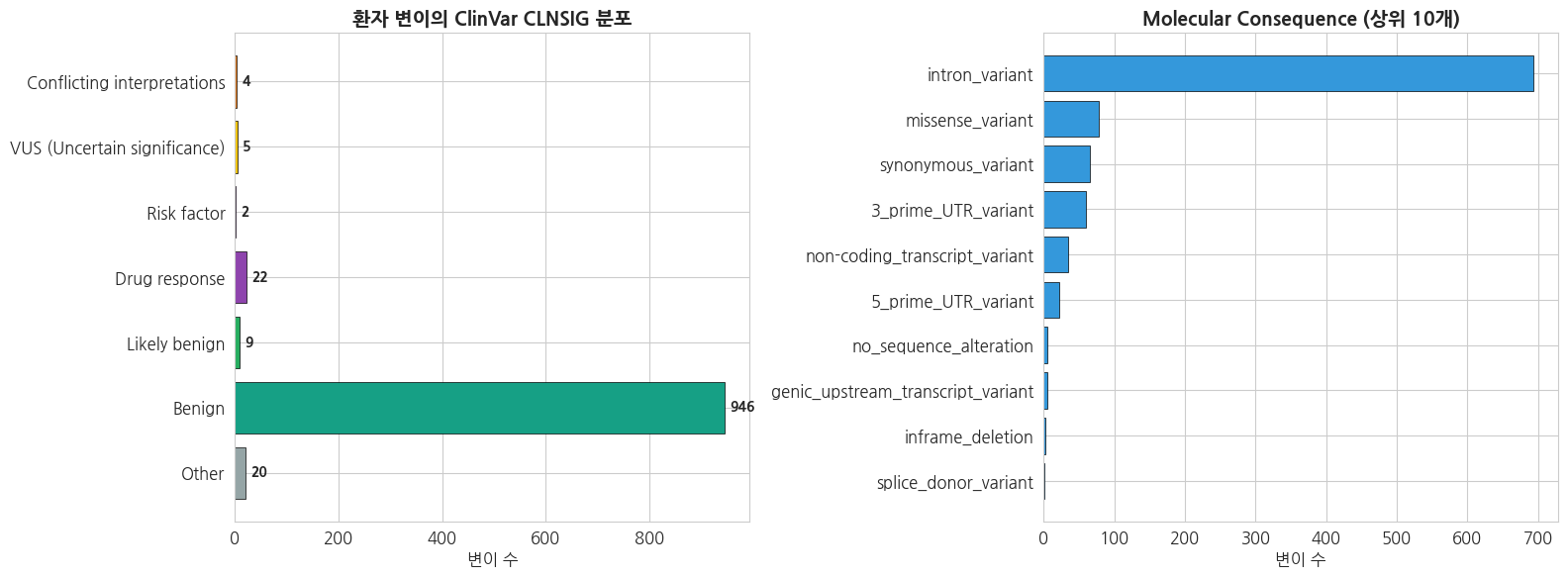

png

3.2 Review Status (증거 수준) 해석

ClinVar의 CLNREVSTAT 는 분류의 근거 강도를 나타냅니다. 높은 신뢰도의 변이를 우선 검토해야 합니다.

Review Status	Stars	설명
practice_guideline	★★★★	임상 지침
reviewed_by_expert_panel	★★★	전문가 패널 리뷰
criteria_provided,_multiple_submitters,_no_conflicts	★★	여러 제출자, 충돌 없음
criteria_provided,_single_submitter	★	단일 제출자
no_assertion_criteria_provided	(없음)	근거 부족

python

# Review Status 별 분포
rev_counts = ann_df['CLNREVSTAT'].value_counts().head(8)
print('=== 환자 변이의 Review Status 분포 ===')
for k, v in rev_counts.items():
    print(f'  {str(k)[:55]:55s}: {v:>6,}')

# 병원성 변이만 Review Status 별로 확인
path_df = ann_df[ann_df['CLNSIG_group'].isin(['Pathogenic', 'Likely pathogenic'])]
print(f'\n=== Pathogenic/Likely pathogenic 변이 ({len(path_df)}개)의 Review Status ===')
print(path_df['CLNREVSTAT'].value_counts())

=== 환자 변이의 Review Status 분포 ===
  criteria_provided,_multiple_submitters,_no_conflicts   :    633
  criteria_provided,_single_submitter                    :    330
  no_assertion_criteria_provided                         :     39
  criteria_provided,_conflicting_classifications         :      4
  reviewed_by_expert_panel                               :      1
  no_classification_provided                             :      1

=== Pathogenic/Likely pathogenic 변이 (0개)의 Review Status ===
Series([], Name: count, dtype: int64)

4. 질환 관련 변이 선별 및 Variant Prioritization

임상 해석에서는 수만 개의 변이 중 실제로 질환과 관련될 가능성이 높은 소수의 후보 변이를 골라내는 것이 핵심입니다.

4.1 Prioritization 일반 전략

일반적인 우선순위화 파이프라인은 다음 필터를 단계적으로 적용합니다:

Quality filter — PASS 변이, 적절한 depth/GQ
Population frequency filter — Rare variant (AF < 1%)
Functional impact filter — HIGH/MODERATE consequence
Clinical database filter — ClinVar Pathogenic/Likely pathogenic
Gene panel filter — 해당 질환 관련 유전자 목록

python

# 단계별 필터링 파이프라인 (환자 전체 변이 기준)
steps = {}

# Step 0: 전체 환자 변이
steps['0. 전체 환자 변이'] = n_patient

# Step 1: ClinVar 주석 있는 변이
steps['1. ClinVar 주석 있음'] = len(ann_df)

# Step 2: Rare variant (ClinVar 변이 중 COMMON=0 또는 RS 기반 - 여기서는 AF_TGP 확인 불가하므로 개념 유지)
# 간략화: Benign/Likely benign 제외
step2 = ann_df[~ann_df['CLNSIG_group'].isin(['Benign', 'Likely benign'])]
steps['2. Benign/LB 제외'] = len(step2)

# Step 3: Functional impact (coding 영역)
coding_consequences = {
    'missense_variant', 'stop_gained', 'stop_lost', 'start_lost',
    'frameshift_variant', 'inframe_insertion', 'inframe_deletion',
    'splice_acceptor_variant', 'splice_donor_variant', 'splice_region_variant',
    'nonsense', 'initiator_codon_variant'
}
step3 = step2[step2['CONSEQUENCE'].isin(coding_consequences)]
steps['3. Coding impact만'] = len(step3)

# Step 4: Pathogenic/Likely pathogenic
step4 = step3[step3['CLNSIG_group'].isin(['Pathogenic', 'Likely pathogenic'])]
steps['4. P / LP'] = len(step4)

# Step 5: Review status ≥ 1 star (criteria_provided)
step5 = step4[step4['CLNREVSTAT'].fillna('').str.contains('criteria_provided', na=False)]
steps['5. ≥ 1 star'] = len(step5)

print('=== 단계별 Variant Prioritization 결과 ===')
for name, count in steps.items():
    print(f'  {name:30s}: {count:>10,}')

prioritized = step5.copy()
print(f'\n→ 최종 우선순위 변이: {len(prioritized)}개')

=== 단계별 Variant Prioritization 결과 ===
  0. 전체 환자 변이                   :     56,754
  1. ClinVar 주석 있음              :      1,008
  2. Benign/LB 제외               :         53
  3. Coding impact만             :          6
  4. P / LP                     :          0
  5. ≥ 1 star                   :          0

→ 최종 우선순위 변이: 0개

python

# 필터링 파이프라인 시각화 (funnel)
_steps_safe = safe_top(steps, n=30)
fig, ax = plt.subplots(figsize=(12, 6), dpi=100)

names = list(_steps_safe.keys())
counts = list(_steps_safe.values())
colors = plt.cm.Reds_r(np.linspace(0.1, 0.8, max(len(names), 1)))

bars = ax.barh(names, counts, color=colors, edgecolor='black', linewidth=0.5)
ax.set_title('Variant Prioritization Funnel', fontsize=14, fontweight='bold')
ax.set_xlabel('변이 수 (log scale)')
ax.set_xscale('symlog')
ax.invert_yaxis()

for bar, val in zip(bars, counts):
    if val > 0:
        ax.text(bar.get_width() * 1.1 + 0.5, bar.get_y() + bar.get_height()/2,
                f'{val:,}', va='center', fontweight='bold', fontsize=10)

fig.tight_layout()
plt.show()
plt.close(fig)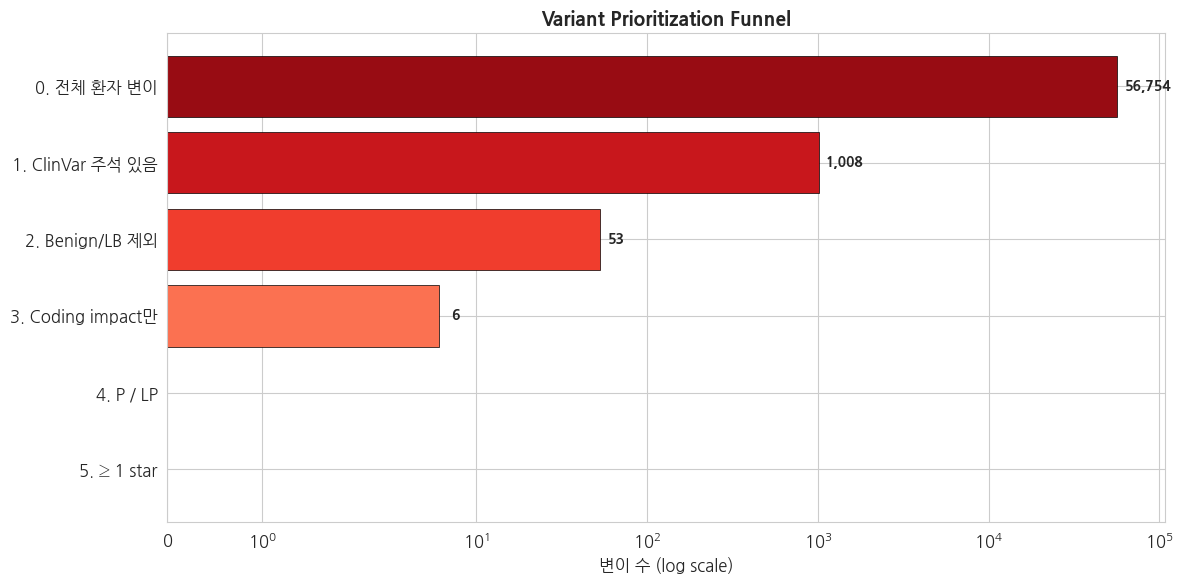

png

4.2 최종 후보 변이 상세 정보

Prioritization으로 선별된 변이를 임상 보고서 형식으로 출력합니다.

python

# 최종 후보 변이 상세 정보
if len(prioritized) == 0:
    print('최종 후보 변이가 없습니다. 임계값을 완화해 재시도하겠습니다.')
    # P/LP 변이만 (star 조건 제외) 다시 사용
    prioritized = step4.copy()

print(f'=== 환자 {target_sample} - 최종 후보 변이 ({len(prioritized)}개) ===\n')

for i, row in prioritized.head(10).reset_index(drop=True).iterrows():
    print(f'[Variant {i+1}]')
    print(f'  위치        : {row["CHROM"]}:{row["POS"]} {row["REF"]}>{row["ALT"]}  ({row["rsID"]})')
    print(f'  유전자      : {row["GENE"]}')
    print(f'  Consequence : {row["CONSEQUENCE"]}')
    print(f'  CLNSIG      : {row["CLNSIG_group"]}  ({row["CLNSIG"]})')
    print(f'  Review      : {row["CLNREVSTAT"]}')
    print(f'  질환        : {str(row["CLNDN"])[:100]}')
    print(f'  Zygosity    : {row["ZYGOSITY"]}')
    print()

최종 후보 변이가 없습니다. 임계값을 완화해 재시도하겠습니다.
=== 환자 NA18939 - 최종 후보 변이 (0개) ===

4.3 질환 관련 유전자별 변이 분포

Pathogenic / Likely pathogenic 변이가 어느 유전자에 집중되는지 확인합니다.

python

# Pathogenic/Likely pathogenic 변이의 유전자 분포
plp_df = ann_df[ann_df['CLNSIG_group'].isin(['Pathogenic', 'Likely pathogenic'])]
gene_counts = plp_df['GENE'].value_counts().head(15)

fig, axes = plt.subplots(1, 2, figsize=(16, 6), dpi=100)

axes[0].barh(gene_counts.index[::-1], gene_counts.values[::-1],
             color='#c0392b', edgecolor='black', linewidth=0.5)
axes[0].set_title(f'P/LP 변이가 있는 Top 15 유전자 (chr22)', fontsize=14, fontweight='bold')
axes[0].set_xlabel('환자 변이 수')

# 전체 환자 변이 vs P/LP 변이 zygosity 비교
zyg_all = ann_df['ZYGOSITY'].value_counts()
zyg_plp = plp_df['ZYGOSITY'].value_counts()

x = np.arange(3)
width = 0.35
categories = ['het', 'hom_alt', 'hom_ref']
all_vals = [zyg_all.get(c, 0) for c in categories]
plp_vals = [zyg_plp.get(c, 0) for c in categories]

# 비율로 비교
all_pct = [v/sum(all_vals)*100 for v in all_vals]
plp_pct = [v/sum(plp_vals)*100 if sum(plp_vals) else 0 for v in plp_vals]

axes[1].bar(x - width/2, all_pct, width, label='전체 주석 변이', color='#3498db', edgecolor='black')
axes[1].bar(x + width/2, plp_pct, width, label='P/LP 변이', color='#c0392b', edgecolor='black')
axes[1].set_xticks(x)
axes[1].set_xticklabels(categories)
axes[1].set_ylabel('비율 (%)')
axes[1].set_title('Zygosity 분포 비교', fontsize=14, fontweight='bold')
axes[1].legend()

fig.tight_layout()
plt.show()
plt.close(fig)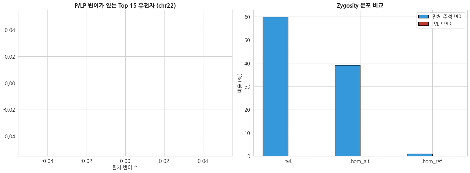

png

5. 암(Somatic) · 희귀질환(Germline) 해석 차이 비교

지금까지 4장 까지는 Germline(NA18939) 환자의 희귀질환 해석 파이프라인을 수행했습니다. 이 장에서는 별도의 공공 데이터인 HCC1395 유방암 세포주의 somatic VCF 를 추가로 분석하여, 두 해석 전략이 실제로 어떻게 다른지 실 데이터로 비교합니다.

5.1 두 해석 전략의 근본적 차이

항목	Germline (희귀질환)	Somatic (암)
변이 기원	생식세포 → 모든 세포에 존재	체세포 → 종양 세포에만 존재
샘플 구성	환자 단일 VCF	Tumor + Normal paired VCF
분석 대상	Rare, 고침투 변이	Somatic mutation (VAF 다양)
Allele Frequency	0.5 (het) / 1.0 (hom)	0.0 ~ 1.0 (종양 clone에 따라)
주요 DB	ClinVar, OMIM, gnomAD	COSMIC, OncoKB, CIViC
분류 guideline	ACMG PVS1, PS, PM, PP, BS, BP	AMP/ASCO/CAP Tier I-IV
임상 질문	"진단 확정이 가능한가?"	"치료 타깃 / 예후 마커는?"
원인 변이 수	1~2개 (단일 유전자 질환)	수십~수천 개 (동반 돌연변이)

5.2 Somatic 실습 데이터: HCC1395

본 실습의 Somatic 트랙에는 SEQC2 consortium 의 HCC1395 high-confidence somatic call set 을 사용합니다. HCC1395 는 유방암 연구에서 표준 벤치마크로 사용되는 세포주입니다.

항목	내용
Cell line	HCC1395 (ATCC CRL-2324)
Matched normal	HCC1395BL (EBV-transformed B-lymphoblast)
원 환자 정보	43세 여성 (Caucasian), primary ductal carcinoma (TNBC)
VCF 출처	NCBI SEQC2 Somatic_Mutation_WG release v1.2.1
Reference	GRCh38
Callers	다중 aligner(BWA/Bowtie/Novo) × 다중 caller 합의 (SomaticSeq)
검증	HighConf / MedConf / LowConf 분류, PacBio long-read 검증 포함

⚠️ Reference genome 차이: Germline 데이터는 GRCh37, Somatic 데이터는 GRCh38 입니다. 실제 임상에서도 다른 연구 데이터가 섞여 올 때 자주 발생하는 이슈입니다. 본 실습은 두 트랙을 각자의 reference 에 맞는 ClinVar 로 독립 annotation 한 뒤, 해석 결과 단계에서 비교합니다.

python

# HCC1395 Somatic VCF 기본 통계
print('=== HCC1395 Somatic VCF 구조 ===')
# 헤더 요약
r = subprocess.run(['bcftools', 'view', '-h', SOMATIC_VCF], capture_output=True, text=True)
hdr = r.stdout.split('\n')
print(f'헤더 라인 수: {len(hdr)}')
print('\nReference:')
for l in hdr:
    if l.startswith('##reference'):
        print(f'  {l}')
        break

# 주요 INFO 필드 (somatic 특이적)
print('\n주요 INFO 필드:')
for l in hdr:
    if l.startswith('##INFO'):
        for key in ['TVAF', 'NVAF', 'bwaClassification', 'nPASSES', 'SOMATIC']:
            if f'ID={key},' in l:
                desc = re.search(r'Description="([^"]+)"', l)
                print(f'  [{key:20s}] {desc.group(1) if desc else ""}')

# 변이 수
r = subprocess.run(['bcftools', 'view', '-H', SOMATIC_VCF], capture_output=True, text=True)
lines = [l for l in r.stdout.strip().split('\n') if l]
n_total = len(lines)

# SNV / INDEL 분리 카운트
n_snv = sum(1 for l in lines if len(l.split('\t')[3]) == 1 and len(l.split('\t')[4]) == 1)
n_indel = n_total - n_snv

# Confidence 레벨
n_highconf = sum(1 for l in lines if 'HighConf' in l.split('\t')[6])
n_medconf  = sum(1 for l in lines if 'MedConf'  in l.split('\t')[6])

print(f'\n=== HCC1395 chr22 변이 통계 ===')
print(f'  총 변이 수     : {n_total:,}')
print(f'  SNV           : {n_snv:,}')
print(f'  INDEL         : {n_indel:,}')
print(f'  HighConf 변이 : {n_highconf:,}')
print(f'  MedConf 변이  : {n_medconf:,}')

=== HCC1395 Somatic VCF 구조 ===
헤더 라인 수: 96

Reference:
  ##reference=file:/SEQC2_Resources/GRCh38.d1.vd1.fa

주요 INFO 필드:
  [TVAF                ] tumor VAF combining 3 aligners
  [NVAF                ] normal VAF combining 3 aligners
  [nPASSES             ] number of samples where the variant is classified as PASS by SomaticSeq
  [bwaClassification   ] bwa-centric classification: Strong, Weak, Neutral, or Likely False Positive based on bwa-aligned data sets
  [SOMATIC             ] Denotes somatic mutation

=== HCC1395 chr22 변이 통계 ===
  총 변이 수     : 657
  SNV           : 627
  INDEL         : 30
  HighConf 변이 : 616
  MedConf 변이  : 41

5.3 Tumor VAF (TVAF) 분포 — Somatic 특이 지표

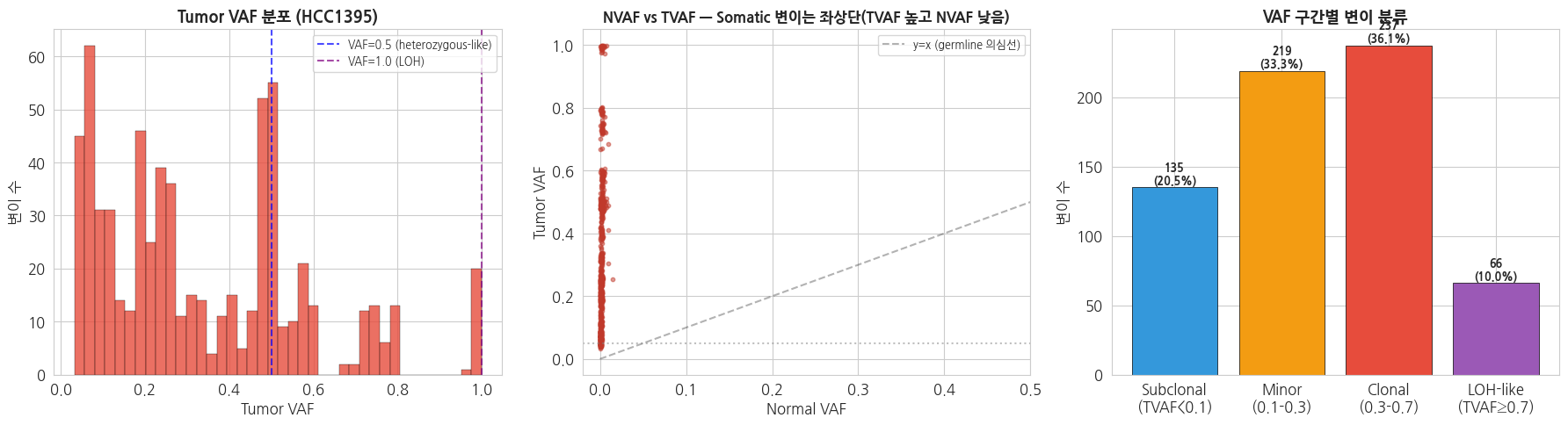
VAF (Variant Allele Frequency) 는 somatic 변이 해석의 핵심 지표입니다.

VAF ≈ 0.5 → 초기 driver mutation 또는 germline 오염 의심
VAF ≈ 1.0 → Loss of heterozygosity (LOH), tumor purity 100%
VAF 낮음 (< 0.1) → Subclonal mutation, 종양 내 이질성 (heterogeneity)
VAF ~ NVAF → 실제로는 germline 변이일 가능성

Germline 변이는 0/0.5/1.0 세 값 근처에 몰리는 반면, Somatic 변이는 연속 분포를 이룹니다. 이것이 두 변이 유형의 가장 큰 차이입니다.

python

# Somatic VCF 파싱 - TVAF, NVAF, FILTER 수집
somatic_records = []

vcf = VCF(SOMATIC_VCF)
for v in vcf:
    tvaf = v.INFO.get('TVAF')
    nvaf = v.INFO.get('NVAF')
    bwa_class = v.INFO.get('bwaClassification')
    n_passes = v.INFO.get('nPASSES')
    flt = v.FILTER if v.FILTER else 'PASS'

    var_type = 'SNV' if (len(v.REF) == 1 and len(v.ALT[0]) == 1) else 'INDEL'

    somatic_records.append({
        'CHROM': v.CHROM,
        'POS': v.POS,
        'REF': v.REF,
        'ALT': v.ALT[0] if v.ALT else '.',
        'FILTER': flt,
        'VAR_TYPE': var_type,
        'TVAF': tvaf,
        'NVAF': nvaf,
        'nPASSES': n_passes,
        'bwaClassification': bwa_class,
    })
vcf.close()

somatic_df = pd.DataFrame(somatic_records)
print(f'Somatic 변이: {len(somatic_df):,}')
print(f'\n=== TVAF / NVAF 기초 통계 ===')
print(somatic_df[['TVAF', 'NVAF']].describe().round(3))

# TVAF 분포 시각화
fig, axes = plt.subplots(1, 3, figsize=(18, 5))

# 1. TVAF 히스토그램
tvaf_valid = somatic_df['TVAF'].dropna()
axes[0].hist(tvaf_valid, bins=40, color='#e74c3c', edgecolor='black',
             linewidth=0.3, alpha=0.8)
axes[0].axvline(0.5, color='blue', linestyle='--', alpha=0.7,
                label='VAF=0.5 (heterozygous-like)')
axes[0].axvline(1.0, color='purple', linestyle='--', alpha=0.7,
                label='VAF=1.0 (LOH)')
axes[0].set_title('Tumor VAF 분포 (HCC1395)', fontsize=13, fontweight='bold')
axes[0].set_xlabel('Tumor VAF')
axes[0].set_ylabel('변이 수')
axes[0].legend(fontsize=9)

# 2. NVAF vs TVAF scatter
axes[1].scatter(somatic_df['NVAF'], somatic_df['TVAF'],
                s=10, alpha=0.5, c='#c0392b')
axes[1].plot([0, 1], [0, 1], 'k--', alpha=0.3, label='y=x (germline 의심선)')
axes[1].axhline(0.05, color='gray', linestyle=':', alpha=0.5)
axes[1].set_xlabel('Normal VAF')
axes[1].set_ylabel('Tumor VAF')
axes[1].set_title('NVAF vs TVAF — Somatic 변이는 좌상단(TVAF 높고 NVAF 낮음)', fontsize=12, fontweight='bold')
axes[1].set_xlim(-0.02, 0.5)
axes[1].legend(fontsize=9)

# 3. VAF 구간별 분류 (Clonal / Subclonal)
vaf_bins = {
    'Subclonal\n(TVAF<0.1)': (somatic_df['TVAF'] < 0.1).sum(),
    'Minor\n(0.1-0.3)': ((somatic_df['TVAF'] >= 0.1) & (somatic_df['TVAF'] < 0.3)).sum(),
    'Clonal\n(0.3-0.7)': ((somatic_df['TVAF'] >= 0.3) & (somatic_df['TVAF'] < 0.7)).sum(),
    'LOH-like\n(TVAF≥0.7)': (somatic_df['TVAF'] >= 0.7).sum(),
}
names = list(vaf_bins.keys())
vals  = list(vaf_bins.values())
colors = ['#3498db', '#f39c12', '#e74c3c', '#9b59b6']
bars = axes[2].bar(names, vals, color=colors, edgecolor='black', linewidth=0.5)
axes[2].set_title('VAF 구간별 변이 분류', fontsize=13, fontweight='bold')
axes[2].set_ylabel('변이 수')
for bar, v in zip(bars, vals):
    axes[2].text(bar.get_x() + bar.get_width()/2, bar.get_height() + max(vals)*0.01,
                 f'{v}\n({v/len(somatic_df)*100:.1f}%)',
                 ha='center', fontsize=9, fontweight='bold')

plt.tight_layout()
plt.show()

Somatic 변이: 657

=== TVAF / NVAF 기초 통계 ===
          TVAF     NVAF
count  657.000  657.000
mean     0.336    0.002
std      0.239    0.002
min      0.032    0.000
25%      0.120    0.000
50%      0.259    0.001
75%      0.494    0.002
max      0.999    0.015

png

5.4 Somatic 변이에 ClinVar GRCh38 annotation

Germline 환자와 동일한 파이프라인이지만, GRCh38 버전 ClinVar 를 사용하고 somatic prioritization 관점으로 해석합니다.

Germline: Pathogenic 이 중요 → 진단 확정
Somatic: Oncogene/TSG 에 위치한 기능적 변이 가 중요 → 표적 치료 탐색

python

# Somatic VCF 에 ClinVar GRCh38 annotation
somatic_annotated = f'{WORK_DIR}/HCC1395_somatic.clinvar.chr22.vcf.gz'

cmd = [
    'bcftools', 'annotate',
    '-a', CLINVAR_GRCH38,
    '-c', 'INFO/CLNSIG,INFO/CLNDN,INFO/CLNREVSTAT,INFO/GENEINFO,INFO/MC,INFO/ORIGIN',
    '-Oz', '-o', somatic_annotated,
    SOMATIC_VCF
]
r = subprocess.run(cmd, capture_output=True, text=True)
subprocess.run(['tabix', '-p', 'vcf', '-f', somatic_annotated],
               capture_output=True, text=True)
print(f'Somatic ClinVar annotation 완료: rc={r.returncode}')

# 주석된 somatic 변이 파싱
s_records = []
vcf = VCF(somatic_annotated)
for v in vcf:
    clnsig = v.INFO.get('CLNSIG')
    gene = v.INFO.get('GENEINFO')
    gene_sym = gene.split(':')[0] if gene else None
    mc = v.INFO.get('MC')
    consequence = None
    if mc:
        for token in mc.split(','):
            if '|' in token:
                consequence = token.split('|')[1]
                break
    s_records.append({
        'CHROM': v.CHROM,
        'POS': v.POS,
        'REF': v.REF,
        'ALT': v.ALT[0] if v.ALT else '.',
        'TVAF': v.INFO.get('TVAF'),
        'NVAF': v.INFO.get('NVAF'),
        'FILTER': v.FILTER if v.FILTER else 'PASS',
        'GENE': gene_sym,
        'CLNSIG': clnsig,
        'CLNDN': v.INFO.get('CLNDN'),
        'CONSEQUENCE': consequence,
    })
vcf.close()

som_ann_df = pd.DataFrame(s_records)

# ClinVar 주석 유무
n_in_clinvar = som_ann_df['CLNSIG'].notna().sum()
print(f'\nHCC1395 chr22 {len(som_ann_df):,}개 변이 중 ClinVar 등록 변이: {n_in_clinvar:,}')
print('(Somatic 변이는 ClinVar 보다 COSMIC/OncoKB 에 많이 등록되어 있음 - 교육상 ClinVar 만 사용)')
print('\n=== ClinVar 에 등록된 Somatic 변이 ===')
print(som_ann_df[som_ann_df['CLNSIG'].notna()].to_string(index=False))

Somatic ClinVar annotation 완료: rc=0

HCC1395 chr22 657개 변이 중 ClinVar 등록 변이: 2
(Somatic 변이는 ClinVar 보다 COSMIC/OncoKB 에 많이 등록되어 있음 - 교육상 ClinVar 만 사용)

=== ClinVar 에 등록된 Somatic 변이 ===
CHROM      POS REF ALT  TVAF  NVAF        FILTER    GENE                 CLNSIG                                                 CLNDN        CONSEQUENCE
   22 29141977   G   A 0.492 0.001 PASS;HighConf KREMEN1                 Benign not_provided|Ectodermal_dysplasia_13,_hair/tooth_type synonymous_variant
   22 46257699   G   A 0.265 0.002 PASS;HighConf  PKDREJ Uncertain_significance                                         not_specified   missense_variant

5.5 Somatic Prioritization — 암 driver 유전자 기반

Somatic 해석은 암 driver gene 에 위치한 기능적 변이를 찾는 것이 핵심입니다. chr22 에 위치한 대표적인 oncogene/TSG 중심으로 prioritization 을 수행합니다.

AMP/ASCO/CAP Tier 기반 분류 (간이 적용)

Tier I: FDA 승인 치료제 타깃 (e.g. BRAF V600E)
Tier II: 가이드라인/임상시험 근거
Tier III: VUS — 임상적 의미 불명
Tier IV: Benign / Likely benign

python

# chr22 에 위치한 대표적 암 유전자 (COSMIC Cancer Gene Census 기반, chr22 일부)
cancer_genes_chr22 = [
    'NF2',      # Neurofibromatosis type 2 (tumor suppressor)
    'CHEK2',    # DNA damage response (tumor suppressor)
    'EWSR1',    # Ewing sarcoma fusion partner
    'MAPK1',    # ERK2 signaling (oncogene)
    'PDGFB',    # Platelet-derived growth factor (oncogene)
    'BCR',      # BCR-ABL fusion (CML)
    'SMARCB1',  # SWI/SNF complex (tumor suppressor)
    'MN1',      # Meningioma-related
    'EP300',    # Histone acetyltransferase (tumor suppressor)
    'NF2', 'SF3B1', 'TCF7L2',
]

# HCC1395 변이 중 암 유전자에 위치한 것 필터링 (GENE 주석은 ClinVar 로부터 온 것이므로 주변 확장 검색 시도)
# VEP REST 를 써서 모든 HCC1395 변이에 gene symbol 부착 (chr22 657개 - 5변이씩 배치)
import json as _json
import requests

VEP_URL_38 = 'https://rest.ensembl.org/vep/human/region'

def annotate_with_vep_rest(df, chunk_size=200):
    """VEP REST (GRCh38) 로 gene symbol + consequence 가져오기"""
    headers = {'Content-Type': 'application/json', 'Accept': 'application/json'}
    results = []
    for i in range(0, len(df), chunk_size):
        chunk = df.iloc[i:i + chunk_size]
        payload = {'variants': [
            f'{r.CHROM} {r.POS} . {r.REF} {r.ALT} . . .'
            for r in chunk.itertuples()
        ]}
        try:
            r = requests.post(VEP_URL_38, headers=headers,
                              data=_json.dumps(payload), timeout=60)
            if r.status_code == 200:
                results.extend(r.json())
            else:
                print(f'  chunk {i}: HTTP {r.status_code}')
        except Exception as e:
            print(f'  chunk {i} 오류: {e}')
    return results

# HighConf 변이만 대상으로 VEP annotation (657개 → 약 3 chunks)
highconf_df = som_ann_df[som_ann_df['FILTER'].apply(
    lambda f: 'HighConf' in (f if isinstance(f, str) else ','.join(f) if f else ''))].copy()
# cyvcf2 FILTER 는 문자열로 반환되므로 간단히 재검사
highconf_df = som_ann_df[som_ann_df['FILTER'].astype(str).str.contains('HighConf', na=False)].copy()
print(f'HighConf 변이: {len(highconf_df)}/{len(som_ann_df)} — VEP REST annotation 수행')

vep_res = annotate_with_vep_rest(highconf_df)
print(f'VEP 응답 수: {len(vep_res)}')

# gene_symbol / consequence 추출
def pick_best(tc_list):
    if not tc_list:
        return {}
    canonical = [t for t in tc_list if t.get('canonical') == 1]
    return (canonical[0] if canonical else tc_list[0])

vep_lookup = {}
for item in vep_res:
    best = pick_best(item.get('transcript_consequences', []))
    vep_lookup[(str(item.get('seq_region_name')), int(item.get('start')))] = {
        'gene_symbol': best.get('gene_symbol'),
        'impact': best.get('impact'),
        'most_severe': item.get('most_severe_consequence'),
    }

# highconf_df 에 VEP 결과 merge
highconf_df['vep_gene']    = highconf_df.apply(
    lambda r: vep_lookup.get((str(r['CHROM']), r['POS']), {}).get('gene_symbol'), axis=1)
highconf_df['vep_impact']  = highconf_df.apply(
    lambda r: vep_lookup.get((str(r['CHROM']), r['POS']), {}).get('impact'), axis=1)
highconf_df['vep_severe']  = highconf_df.apply(
    lambda r: vep_lookup.get((str(r['CHROM']), r['POS']), {}).get('most_severe'), axis=1)

# 암 유전자 필터링
cancer_hits = highconf_df[highconf_df['vep_gene'].isin(set(cancer_genes_chr22))]
print(f'\n=== HCC1395 의 암 유전자 변이 (chr22, HighConf) ===')
print(f'암 유전자 후보: {len(cancer_hits)}')
if len(cancer_hits):
    cols = ['CHROM', 'POS', 'REF', 'ALT', 'TVAF', 'NVAF',
            'vep_gene', 'vep_severe', 'vep_impact']
    print(cancer_hits[cols].to_string(index=False))
else:
    print('(해당 없음 — chr22 는 암 유전자 hotspot 이 상대적으로 적음)')

# 기능 영향 기반 순위 (HIGH/MODERATE 만)
functional_hits = highconf_df[highconf_df['vep_impact'].isin(['HIGH', 'MODERATE'])].copy()
functional_hits = functional_hits.sort_values('TVAF', ascending=False)
print(f'\n=== HighConf + Coding impact (HIGH/MODERATE) 변이 — 상위 10 ===')
cols = ['CHROM', 'POS', 'REF', 'ALT', 'TVAF', 'vep_gene',
        'vep_severe', 'vep_impact']
print(functional_hits[cols].head(10).to_string(index=False))

HighConf 변이: 616/657 — VEP REST annotation 수행
VEP 응답 수: 616

=== HCC1395 의 암 유전자 변이 (chr22, HighConf) ===
암 유전자 후보: 12
CHROM      POS REF ALT  TVAF  NVAF vep_gene                         vep_severe vep_impact
   22 23178829   C   G 0.299 0.002      BCR              upstream_gene_variant   MODIFIER
   22 23237703   G   A 0.108 0.000      BCR                     intron_variant   MODIFIER
   22 23274642   G   A 0.113 0.000      BCR                     intron_variant   MODIFIER
   22 23802508   C   G 0.181 0.001  SMARCB1 non_coding_transcript_exon_variant   MODIFIER
   22 27761963   G   A 0.320 0.002      MN1                     intron_variant   MODIFIER
   22 27778986   T   A 0.087 0.000      MN1                     intron_variant   MODIFIER
   22 28688787   G   C 0.465 0.001    CHEK2                     intron_variant   MODIFIER
   22 28731132   G   A 0.073 0.000    CHEK2                     intron_variant   MODIFIER
   22 29286163   G   A 0.529 0.000    EWSR1                     intron_variant   MODIFIER
   22 39236803   G   A 0.219 0.000    PDGFB                     intron_variant   MODIFIER
   22 41135122   G   A 0.135 0.001    EP300                     intron_variant   MODIFIER
   22 41181018   G   T 0.252 0.000    EP300                     intron_variant   MODIFIER

=== HighConf + Coding impact (HIGH/MODERATE) 변이 — 상위 10 ===
CHROM      POS REF ALT  TVAF vep_gene       vep_severe vep_impact
   22 50177152   C   T 0.998    PANX2 missense_variant   MODERATE
   22 37631021   C   G 0.494     GGA1 missense_variant   MODERATE
   22 37570268   C   G 0.490   LGALS2 missense_variant   MODERATE
   22 46257699   G   A 0.265   PKDREJ missense_variant   MODERATE
   22 41524891   G   C 0.240     ACO2 missense_variant   MODERATE
   22 37374978   G   A 0.161    ELFN2 missense_variant   MODERATE
   22 50210823   G   C 0.089  SELENOO missense_variant   MODERATE
   22 35726447   G   T 0.047    APOL5 missense_variant   MODERATE

5.6 Germline(NA18939) vs Somatic(HCC1395) 해석 결과 비교

두 트랙의 chr22 해석 결과를 한 눈에 비교합니다.

python

# Germline(NA18939) vs Somatic(HCC1395) 비교 시각화
fig, axes = plt.subplots(2, 2, figsize=(16, 10), dpi=100)

# 1. 전체 변이 수
germline_counts = {
    '전체 변이': n_patient,
    'ClinVar 주석': len(ann_df),
    'P/LP': len(plp_df),
}
somatic_counts = {
    '전체 변이': len(som_ann_df),
    'ClinVar 주석': n_in_clinvar,
    'Coding impact\n(HIGH/MOD)': len(functional_hits),
}

x = np.arange(3)
width = 0.35
axes[0, 0].bar(x - width/2, list(germline_counts.values()), width,
                label='Germline (NA18939)', color='#3498db', edgecolor='black')
axes[0, 0].bar(x + width/2, list(somatic_counts.values()), width,
                label='Somatic (HCC1395)', color='#e74c3c', edgecolor='black')
axes[0, 0].set_xticks(x)
axes[0, 0].set_xticklabels(['전체', 'ClinVar\n주석', 'Filter 후\n후보'])
axes[0, 0].set_ylabel('변이 수 (log)')
axes[0, 0].set_yscale('log')
axes[0, 0].set_title('Germline vs Somatic — 변이 수 비교 (chr22)',
                      fontsize=13, fontweight='bold')
axes[0, 0].legend()
for i, (g, s) in enumerate(zip(germline_counts.values(), somatic_counts.values())):
    if g > 0:
        axes[0, 0].text(i - width/2, g, f'{g:,}', ha='center', va='bottom', fontsize=9)
    if s > 0:
        axes[0, 0].text(i + width/2, s, f'{s:,}', ha='center', va='bottom', fontsize=9)

# 2. Allele Frequency 분포 비교 (Germline 0/0.5/1.0 vs Somatic 연속)
germline_af = ann_df['ZYGOSITY'].map({'hom_ref': 0.0, 'het': 0.5, 'hom_alt': 1.0}).dropna()
somatic_af_valid = somatic_df['TVAF'].dropna()
# 수치 이상치 방어: [0, 1] 범위만 사용
somatic_af_valid = somatic_af_valid[(somatic_af_valid >= 0) & (somatic_af_valid <= 1)]

bins = np.linspace(0, 1, 41)
if len(germline_af) > 0:
    axes[0, 1].hist(germline_af, bins=bins, alpha=0.6,
                     label='Germline GT (NA18939)', color='#3498db', edgecolor='black')
if len(somatic_af_valid) > 0:
    axes[0, 1].hist(somatic_af_valid, bins=bins, alpha=0.6,
                     label='Somatic TVAF (HCC1395)', color='#e74c3c', edgecolor='black')
axes[0, 1].set_title('Allele Frequency 분포', fontsize=13, fontweight='bold')
axes[0, 1].set_xlabel('Allele Frequency')
axes[0, 1].set_ylabel('변이 수 (log)')
axes[0, 1].set_yscale('log')
axes[0, 1].set_xlim(0, 1)
axes[0, 1].legend()

# 3. Consequence 분포 비교 (상위 6개)
germline_cons = ann_df['CONSEQUENCE'].dropna().value_counts().head(6)
somatic_cons  = pd.Series([v['most_severe'] for v in vep_lookup.values()
                            if v.get('most_severe')]).value_counts().head(6)

# union 크기 방어: 최대 12개로 제한
all_cons = sorted(set(germline_cons.index) | set(somatic_cons.index))[:12]
g_vals = [germline_cons.get(c, 0) for c in all_cons]
s_vals = [somatic_cons.get(c, 0) for c in all_cons]

y = np.arange(len(all_cons))
height = 0.35
if len(all_cons) > 0:
    axes[1, 0].barh(y - height/2, g_vals, height,
                     label='Germline', color='#3498db', edgecolor='black')
    axes[1, 0].barh(y + height/2, s_vals, height,
                     label='Somatic', color='#e74c3c', edgecolor='black')
    axes[1, 0].set_yticks(y)
    axes[1, 0].set_yticklabels(all_cons, fontsize=9)
axes[1, 0].set_xlabel('변이 수')
axes[1, 0].set_title('Consequence 분포 (상위)', fontsize=13, fontweight='bold')
axes[1, 0].legend()

# 4. 해석의 임상적 초점 요약 (axis 좌표계 사용)
axes[1, 1].axis('off')
axes[1, 1].set_xlim(0, 1)
axes[1, 1].set_ylim(0, 1)
focus_text = (
    "Germline (NA18939)\n"
    "───────────────\n"
    "• 희귀질환 진단 여부\n"
    "• ACMG 분류 (P / LP / VUS / B)\n"
    "• 가족 검사 및 유전상담\n"
    "• DB: ClinVar / OMIM / gnomAD\n\n"
    "Somatic (HCC1395)\n"
    "───────────────\n"
    "• 표적치료제 탐색\n"
    "• AMP Tier I-IV 분류\n"
    "• Tumor clonality (VAF 분포)\n"
    "• DB: COSMIC / OncoKB / CIViC\n"
)
# family='monospace' 제거 → 한글 깨짐 방지 (sans-serif 한글 폰트 사용)
axes[1, 1].text(0.05, 0.5, focus_text, fontsize=11,
                verticalalignment='center',
                transform=axes[1, 1].transAxes)
axes[1, 1].set_title('해석의 임상적 초점', fontsize=13, fontweight='bold')

fig.tight_layout()
plt.show()
plt.close(fig)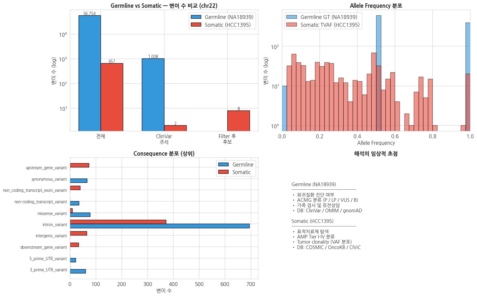

png

5.7 실제 임상 적용 시 체크리스트

단계	Germline 해석	Somatic 해석
1. 샘플	환자 단독 WGS/WES	Tumor + Matched Normal
2. Variant calling	GATK HaplotypeCaller, DeepVariant	Mutect2, Strelka2, VarScan2, SomaticSeq
3. Filtering	Hardy-Weinberg, trio 분석	tumor VAF, Panel of Normal
4. Annotation	VEP + ClinVar + gnomAD	VEP + COSMIC + OncoKB
5. Prioritization	ACMG guideline (P/LP/VUS/LB/B)	AMP/ASCO/CAP Tier I-IV
6. 보고서	진단 확정 + 유전상담	표적치료제 + 임상시험 매칭

6. 결과물 저장 및 요약

python

# Germline prioritized variants 저장
out_path = f'{WORK_DIR}/patient_{target_sample}.prioritized.tsv'
prioritized.to_csv(out_path, sep='\t', index=False)
print(f'[Germline] 우선순위 변이 저장: {out_path}')
print(f'  - 샘플: {target_sample}')
print(f'  - 변이 수: {len(prioritized)}')

# Germline P/LP 변이 저장
germline_out = f'{WORK_DIR}/patient_{target_sample}.germline_plp.tsv'
plp_df.to_csv(germline_out, sep='\t', index=False)
print(f'\n[Germline] P/LP 변이 저장: {germline_out}')
print(f'  - 변이 수: {len(plp_df)}')

# Somatic HighConf + Coding 변이 저장
somatic_out = f'{WORK_DIR}/HCC1395_somatic.prioritized.tsv'
functional_hits.to_csv(somatic_out, sep='\t', index=False)
print(f'\n[Somatic] Functional 변이 저장: {somatic_out}')
print(f'  - 샘플: HCC1395')
print(f'  - 변이 수: {len(functional_hits)}')
print(f'  - 암 유전자 위치 변이: {len(cancer_hits)}')

[Germline] 우선순위 변이 저장: /tier4/DSC/jheepark/bbp-wgs-data/individual/patient_NA18939.prioritized.tsv
  - 샘플: NA18939
  - 변이 수: 0

[Germline] P/LP 변이 저장: /tier4/DSC/jheepark/bbp-wgs-data/individual/patient_NA18939.germline_plp.tsv
  - 변이 수: 0

[Somatic] Functional 변이 저장: /tier4/DSC/jheepark/bbp-wgs-data/individual/HCC1395_somatic.prioritized.tsv
  - 샘플: HCC1395
  - 변이 수: 8
  - 암 유전자 위치 변이: 12

이번 강의 요약

항목	Germline (NA18939)	Somatic (HCC1395)
데이터 출처	1000 Genomes Phase 3	SEQC2 HCC1395 high-confidence callset
Reference	GRCh37	GRCh38
변이 수 (chr22)	~수만개	657개 (SNV 627 + INDEL 30)
주요 INFO	AF, AC (population freq)	TVAF, NVAF, HighConf, PACB 검증
Annotation	ClinVar GRCh37 + VEP	ClinVar GRCh38 + VEP REST
Prioritization	ClinVar → Coding → P/LP → ≥ 1 star	HighConf → Coding (HIGH/MOD) → 암 유전자
임상 기준	ACMG guideline	AMP/ASCO/CAP Tier

핵심 포인트

Annotation 은 VCF 해석의 시작점 — 위치/염기만으로는 임상적 의미를 알 수 없음
ClinVar CLNSIG + CLNREVSTAT 조합으로 신뢰도 높은 병원성 변이 선별
VEP 는 기능적 영향, ClinVar 는 임상적 병원성 — 상호 보완적이므로 두 결과를 함께 검토
Prioritization 은 funnel 구조 — 빈도 → 기능 → 임상 DB → 유전자 순으로 좁혀감
Germline vs Somatic 은 완전히 다른 파이프라인
- Germline: 이산적 VAF (0/0.5/1.0), 전체 세포 공유, ACMG guideline
- Somatic: 연속 VAF 분포 (subclone), 종양 내 heterogeneity, AMP Tier
Reference genome 버전 차이는 실제 임상에서 자주 발생하는 이슈 — bcftools annotate 는 position/REF/ALT 매칭이므로 reference 가 반드시 일치해야 함

주요 명령어 정리

bash

# ClinVar INFO 주입 (Germline)
bcftools annotate \
    -a clinvar.vcf.gz \
    -c INFO/CLNSIG,INFO/CLNDN,INFO/GENEINFO \
    -Oz -o patient.clinvar.vcf.gz \
    patient.vcf.gz

# ClinVar INFO 주입 (Somatic, GRCh38)
bcftools annotate \
    -a clinvar_GRCh38.vcf.gz \
    -c INFO/CLNSIG,INFO/CLNDN,INFO/GENEINFO,INFO/MC,INFO/ORIGIN \
    -Oz -o tumor.clinvar.vcf.gz \
    tumor.vcf.gz

# TVAF 필터링 (Somatic, clonal 만)
bcftools view -i 'INFO/TVAF>=0.3 && INFO/TVAF<=0.7' tumor.clinvar.vcf.gz

# 병원성 변이만 추출 (Germline)
bcftools view -i 'INFO/CLNSIG~"Pathogenic"' patient.clinvar.vcf.gz

python

# VEP REST API (GRCh37 vs GRCh38)
import requests, json
url_37 = 'https://grch37.rest.ensembl.org/vep/human/region'
url_38 = 'https://rest.ensembl.org/vep/human/region'
r = requests.post(url_38,
                  headers={'Content-Type':'application/json', 'Accept':'application/json'},
                  data=json.dumps({'variants':['22 16258221 . C T . . .']}))
print(r.json()[0]['most_severe_consequence'])

다음 강의 예고

4강: 환자 코호트 기반 질병 연관성 분석

다수 환자 VCF 통합 및 코호트 QC 수행
GWAS 분석 실행 및 결과 시각화
PRS(Polygenic Risk Score) 계산을 통한 개인별 유전적 위험도 비교

3강: 개인 환자 유전체 기반 변이 해석 ​

BBP WGS 분석 튜토리얼 ​

학습 목표 ​

사용 데이터 ​

Germline 트랙 (GRCh37) ​

Somatic 트랙 (GRCh38) ​

산출물 (본 강의에서 생성) ​

사용 도구 ​

0. 환경 설정 ​

1. 변이 주석(Annotation) 개요 ​

1.1 Annotation이란? ​

1.2 ClinVar 데이터 구조 ​

2. 개인 환자 샘플 선택 및 변이 주석 ​

2.1 분석 대상 환자 선택 ​

2.2 ClinVar annotation 주입 ​

2.3 Ensembl VEP 설치 및 간단한 Annotation 실습 ​

설치 방법 (3가지 중 택일) ​

① Docker 설치 (권장) ​

② Singularity 설치 (HPC 환경) ​

③ Conda 설치 ​

설치 확인 ​

VEP 주요 Consequence 범주 ​

간단한 VEP Annotation 실습 ​

방법 A — Docker 로 VEP 로컬 실행 (cache 설치된 경우) ​

방법 B — Ensembl REST API 로 즉시 Annotation (cache 불필요) ​

VEP 결과와 ClinVar 결과 비교 ​

3. 주석 결과 파싱 및 해석 ​

3.1 CLNSIG (병원성 분류) 분포 ​

3.2 Review Status (증거 수준) 해석 ​

4. 질환 관련 변이 선별 및 Variant Prioritization ​

4.1 Prioritization 일반 전략 ​

4.2 최종 후보 변이 상세 정보 ​

4.3 질환 관련 유전자별 변이 분포 ​

5. 암(Somatic) · 희귀질환(Germline) 해석 차이 비교 ​

5.1 두 해석 전략의 근본적 차이 ​

5.2 Somatic 실습 데이터: HCC1395 ​

5.3 Tumor VAF (TVAF) 분포 — Somatic 특이 지표 ​

5.4 Somatic 변이에 ClinVar GRCh38 annotation ​

5.5 Somatic Prioritization — 암 driver 유전자 기반 ​

5.6 Germline(NA18939) vs Somatic(HCC1395) 해석 결과 비교 ​

5.7 실제 임상 적용 시 체크리스트 ​

6. 결과물 저장 및 요약 ​

이번 강의 요약 ​

핵심 포인트 ​

주요 명령어 정리 ​

다음 강의 예고 ​

3강: 개인 환자 유전체 기반 변이 해석

BBP WGS 분석 튜토리얼

학습 목표

사용 데이터

Germline 트랙 (GRCh37)

Somatic 트랙 (GRCh38)

산출물 (본 강의에서 생성)

사용 도구

0. 환경 설정

1. 변이 주석(Annotation) 개요

1.1 Annotation이란?

1.2 ClinVar 데이터 구조

2. 개인 환자 샘플 선택 및 변이 주석

2.1 분석 대상 환자 선택

2.2 ClinVar annotation 주입

2.3 Ensembl VEP 설치 및 간단한 Annotation 실습

설치 방법 (3가지 중 택일)

① Docker 설치 (권장)

② Singularity 설치 (HPC 환경)

③ Conda 설치

설치 확인

VEP 주요 Consequence 범주

간단한 VEP Annotation 실습

방법 A — Docker 로 VEP 로컬 실행 (cache 설치된 경우)

방법 B — Ensembl REST API 로 즉시 Annotation (cache 불필요)

VEP 결과와 ClinVar 결과 비교

3. 주석 결과 파싱 및 해석

3.1 CLNSIG (병원성 분류) 분포

3.2 Review Status (증거 수준) 해석

4. 질환 관련 변이 선별 및 Variant Prioritization

4.1 Prioritization 일반 전략

4.2 최종 후보 변이 상세 정보

4.3 질환 관련 유전자별 변이 분포

5. 암(Somatic) · 희귀질환(Germline) 해석 차이 비교

5.1 두 해석 전략의 근본적 차이

5.2 Somatic 실습 데이터: HCC1395

5.3 Tumor VAF (TVAF) 분포 — Somatic 특이 지표

5.4 Somatic 변이에 ClinVar GRCh38 annotation

5.5 Somatic Prioritization — 암 driver 유전자 기반

5.6 Germline(NA18939) vs Somatic(HCC1395) 해석 결과 비교

5.7 실제 임상 적용 시 체크리스트

6. 결과물 저장 및 요약

이번 강의 요약

핵심 포인트

주요 명령어 정리

다음 강의 예고